Lab 1 Optimisation

Topics

• Aims and Objectives
• Overview and Exercise
• Background Information
• Exercise 1: Optimisation

Learning Outcomes

By the end of this lesson, you will be able to:

• Evaluate and visualise a cost function.
• Use different solvers in MATLAB© to solve optimisation problems.
• Solve real world optimisation problems relating to powertrains.

Aims and Objectives

The aim of this exercise is to gain an understanding of basic optimisation approaches, this will be evaluated in the setting of mathematics and engine operation.

Overview of Exercise

The optimisation problem is an abstraction of the problem of making the best possible choices from a set of candidate choices. This includes the representation of the choice made, the constraints (specifications or limits) and the objective function (representing the cost of making a specific choice). The solution of the optimisation problem is the choice that has the minimum cost among all choices that meet the requirements.

Background Information

The MATLAB© Optimisation Toolbox provides functions for finding parameters that minimize or maximize objectives while satisfying constraints. The toolbox includes solvers for linear programming, mixed-integer linear programming, quadratic programming, nonlinear optimisation and nonlinear least squares. You can use these solvers to find optimal solutions to continuous and discrete problems, perform trade-off analyses and incorporate optimisation methods into algorithms and applications. We will use the optimisation GUI as well as code.

Exercise 1: Optimisation

Download the data for this exercise here

Task 1-1: Basics of Optimisation

The file J1.m implements the following nicely shaped cost function:

as a function;

function [cost] = J1(p1,p2)
cost = p1.^2 + exp(p2) + exp(-p2) + p1 .* p2 + p2;

in MATLAB©.

• Evaluate \(J_1\) for a number of points and try to get a feeling for it, you can use a simple call with two arguments such as <J1(arg1,arg2)>.
• Visualise this function. The ez plot functions are convenient to do this, such as <ezsurf(@J1)> or <ezcontour(@J1)>. Which kind of plot is most suitable?

• Use <fminsearch(fun, x0)> to find the minimum starting the search from x0 = [0,0]: <fminsearch(@J1vect,[0, 0])>. The <fminsearch> expects a function with a single vector argument therefore the version defined in J1vect.m has to be used. Try different starting points.
• How many evaluations of \(J\) are required by <fminsearch>?

Task 1-2: Optimtool GUI

The same exercise can be achieved using the graphical interface, which presents more information about the optimisation process.

• Open up the MATLAB© LiveScript GetStartedWithOptimizeLiveEditorTaskExample1.mlx from the files downloaded. This is a generic script so will need to be changed slightly as follows.
• Familiarise yourself with the script in particular the Optimise task.
• Enter the starting point [0 0].
• Select Unconstrained optimisation.
• Select the solver <fminsearch>.
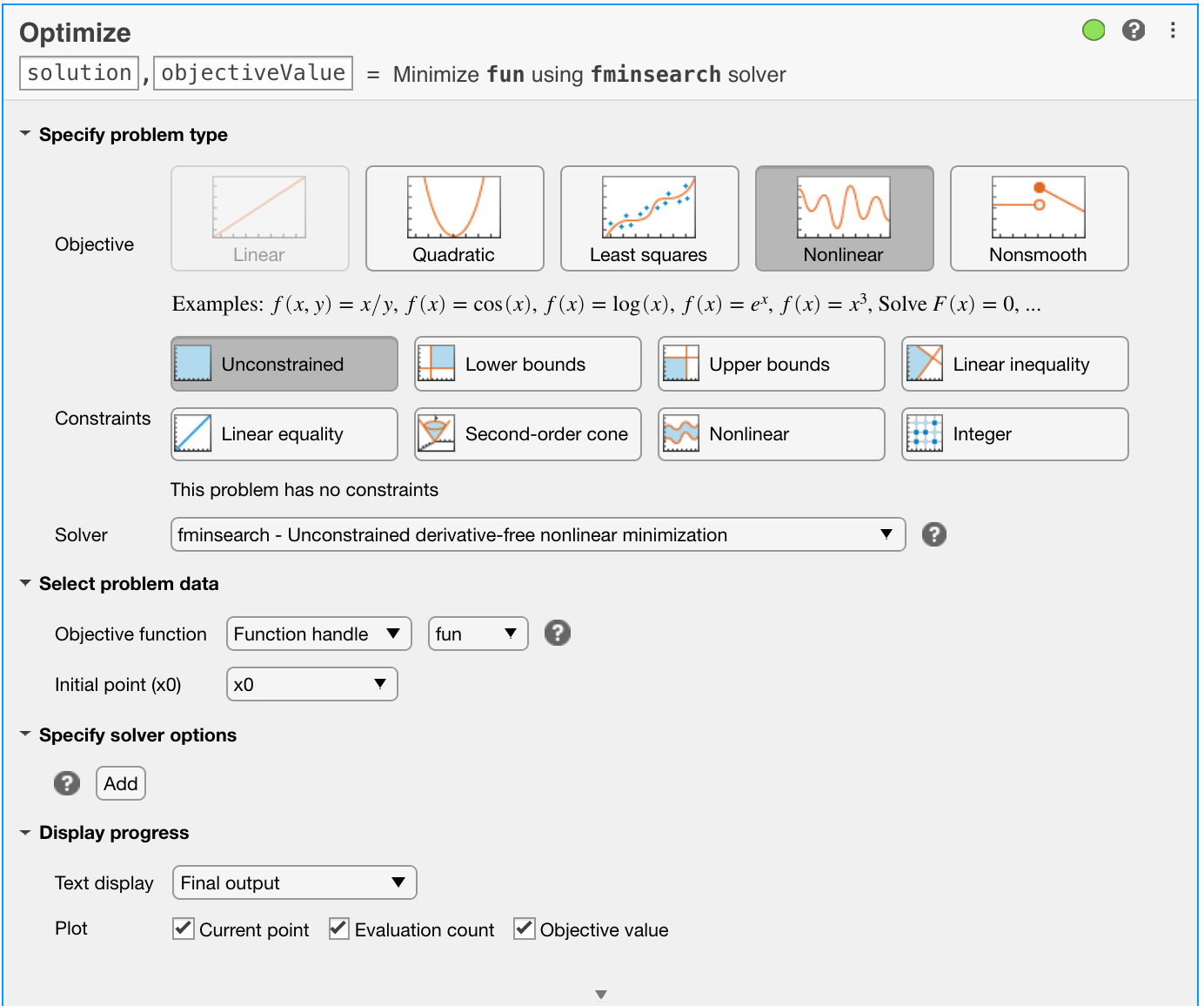
• Enter the objective function <@J1vect> noting that there are a few different ways that this can be done.
• Ensure you have selected the plot options [Current point], [Evaluation count] and [Objective value]. Once you have completed making the changes, the task interface should look like the figure below.

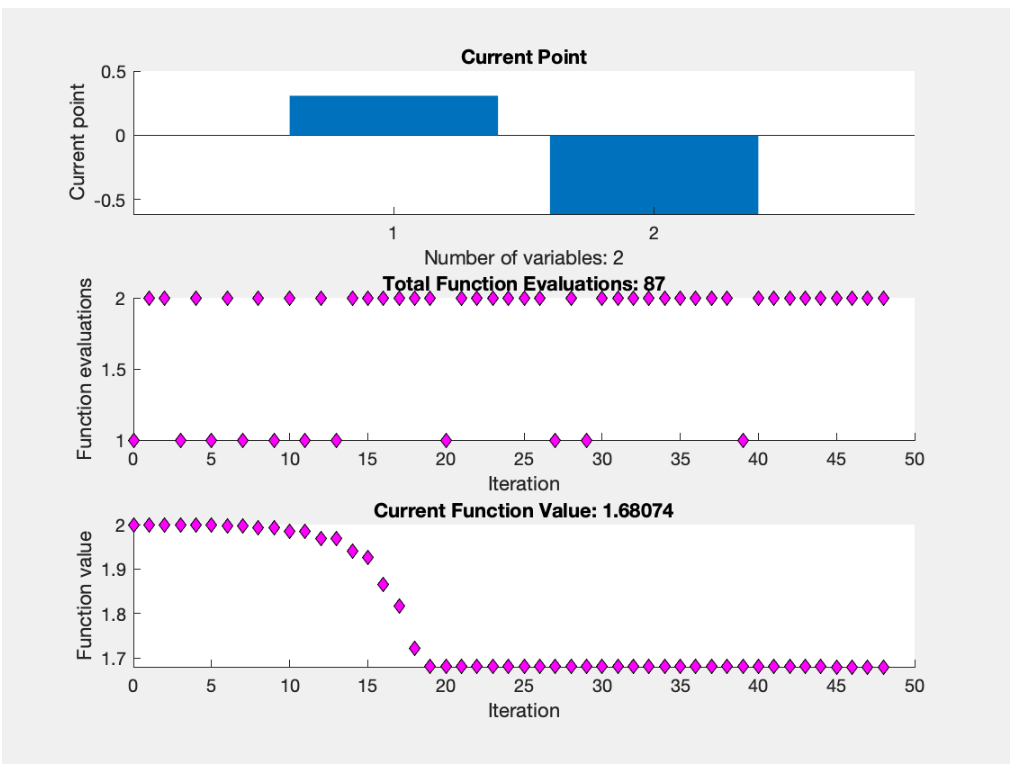
• Under Plot Functions enable the options [Function Count] and [Function Value]. This shows how the function value decreases during the optimisation.
• Click [Run]. How long does it take and how many iterations are required? Your results should look like the figure shown below.

• Try the same with the solver <fminunc>. What is the main difference between this and the previous solver?
• Try a constrained minimisation using the solver <fmincon>. You have to supply bounds for \(p\) such as Lower: \([-10, -10]\) and Upper: \([10, 10]\). What happens if you only allow positive values?

Task 1-3: Optimal Powertrain Calibration

The file model_V8NA_V2.m is a simple model of a naturally aspirated spark ignition V8 engine at a fixed engine speed. It takes a single vector argument with three values: the relative load (0 to 100), the spark advance angle (0 to 35) and the normalised air fuel ratio (0.8 to 1.1). The output is a vector of 6 measurements: BMEP (in bar), SD of BMEP (in bar), exhaust mass flow (in kg/h), exhaust temperature (in C), fuel consumption (in kg/h) and BSFC (in g/kWh).

• For a relative load of 50 and an Air-Fuel Ratio of 1, find the best BSFC. You can use unconstrained optimisation with <fminsearch> or constrained optimisation using <X = fmincon(FUN,X0,A,B)> for this. You will need to write your own cost function that calls the model function.
• A better formulation of this problem is to find the best BSFC for a given BMEP (6 bar as a good example), relative load and air fuel ratio. Use the fixed values of 50 for relative load and 1 for air fuel ratio as in the last question.
• Repeat this optimisation for a number of steps from 1 bar to 10 bar BMEP. This will result in an optimal calibration but is it realistic? Which requirements have been ignored? How could you include them?

Task 1-4: Multicriteria Optimisation (optional)

Consider the following multicriteria cost function. It distinguishes between two stretches driven with different speeds \(p_1\) and \(p_2\);

• Plot the function above. Is it convex?
• Find the optimum for a set of hourly costs \(\alpha\). You have to edit the function J4.m to change \(\alpha\). (If you are a more advanced user of MATLAB© you could automate this process).
• How can the results be visualised? Create a diagram with the key relationships.