Engine Modelling
In this laboratory you will be making use of Simulink to model a naturally aspirated, 5l V8 Jaguar Engine using parameters and data obtained by measurement and test during experimentation.
The aim of the laboratory is to produce a simple air-path model that is capable of estimating engine airflow and torque over the speed range.
This exercise will teach you how a typical airpath/torque model is created within Simulink. These types of mean value models form the backbone of many engine and related simulation-based development efforts. Additionally, it will allow you to develop your expertise within Simulink. Finally, a simplified form of this model will be used during MIRA week.
Approach to the development of the Engine Model
Download the engine model template, EngTemplate.slx from LEARN and open it in Simulink. Also download the model parameters file called EngParameters.m and open these in the editor.

Look at the inputs and outputs of each of the main top-level blocks within the Simulink model, this defines the information available in each of the subsystems; Throttle Body, Intake Manifold and Torque generation. Note the units required for each of these inputs and outputs.
Now look at the model parameters in the parameter file, this represents the information that is known about the engine. Each of these also has a description of the units of the data.
You may wish to refer to the lecture slides on Engine Modelling to help you understand how the model is implemented.
Throttle Body

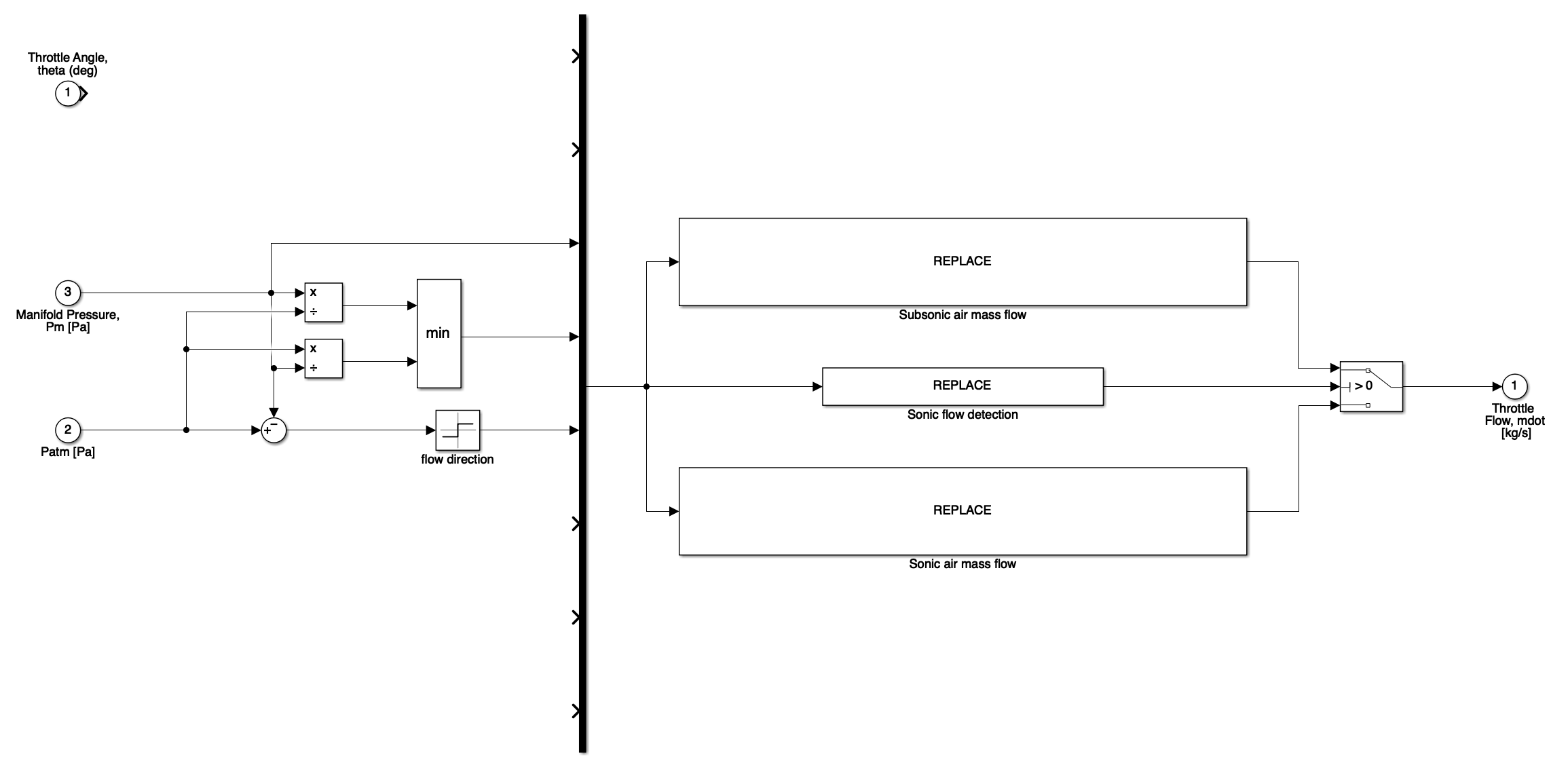
Open the Throttle Body submodel and again note the inputs and outputs available. Recall the equation that describes throttle mass flow is piecewise continuous i.e. the throttle pressure ratio determines if the flow is to be treated as choked or not and hence which equation is required to describe the mass flow through the throttle.
For un-choked flow $\frac{P_{man}}{P_{atm}} > 0.528$;
\[\dot{m}=\frac{C_{d} A_{t h} P_{a t m}}{\sqrt{R T_{a t m}}}\left(\frac{P_{m a n}}{P_{a t m}}\right)^{\frac{1}{\gamma}}\left\{\frac{2 \gamma}{\gamma-1}\left[1-\left(\frac{P_{m a n}}{P_{a t m}}\right)^{\frac{\gamma-1}{\gamma}}\right]\right\}^{\frac{1}{2}} \nonumber\]For choked flow $\frac{P_{man}}{P_{atm}} \leq 0.528$;
\[\dot{m}=\frac{C_{d} A_{th} P_{atm}}{\sqrt{R T_{atm}}} \sqrt{\gamma}\left(\frac{2}{\gamma+1}\right)^{\frac{\gamma+1}{2(\gamma-1)}} \nonumber\]Note that in reverse flow the pressure ratio reverses so that for un-choked flow $\frac{P_{atm}}{P_{man}} > 0.528$;
\[\dot{m}=\frac{C_{d} A_{t h} P_{man}}{\sqrt{R T_{man}}}\left(\frac{P_{atm}}{P_{man}}\right)^{\frac{1}{\gamma}}\left\{\frac{2 \gamma}{\gamma-1}\left[1-\left(\frac{P_{atm}}{P_{man}}\right)^{\frac{\gamma-1}{\gamma}}\right]\right\}^{\frac{1}{2}} \nonumber\]For choked flow $\frac{P_{atm}}{P_{man}} \leq 0.528$;
\[\dot{m}=\frac{C_{d} A_{th} P_{man}}{\sqrt{R T_{man}}} \sqrt{\gamma}\left(\frac{2}{\gamma+1}\right)^{\frac{\gamma+1}{2(\gamma-1)}} \nonumber\]A suggested switching mechanism has been included in the model, make sure you understand how this works. Note carefully how the change of direction in flow is implemented (this is something the equations don’t help you with). A MUX block is used to tidy up the many signals these may be referenced from the output of the MUX block using the notation u[1] to select the first signal, u[2] the second and so on.
Using the equations shown in the lecture slides build the model, the MATLAB version of the throttle area and subsonic flow are included below for your convenience. Remember however that you should check the inputs to this (u(1), u(2), etc) to make sure they are correct according to your implementation.
%throttle area equation
(pi*D^2)/4*((1-cos(u(1))/cos(u0))+2/pi*(a/cos(u(1))*(cos(u(1))^2-a^2*cos(u0)^2)^(1/2)-cos(u(1))/cos(u0)*asin(a*cos(u0)/cos(u(1)))-a*(1-a^2)^(1/2)+asin(a)))

%subsonic flow equation
(((u(1)*u(2)*u(3))/sqrt(u(8)*u(6)))*(u(4)^(1/u(7)))*sqrt((2*u(7)/(u(7)-1))*(1-(u(4)^((u(7)-1)/u(7))))))*u(5)
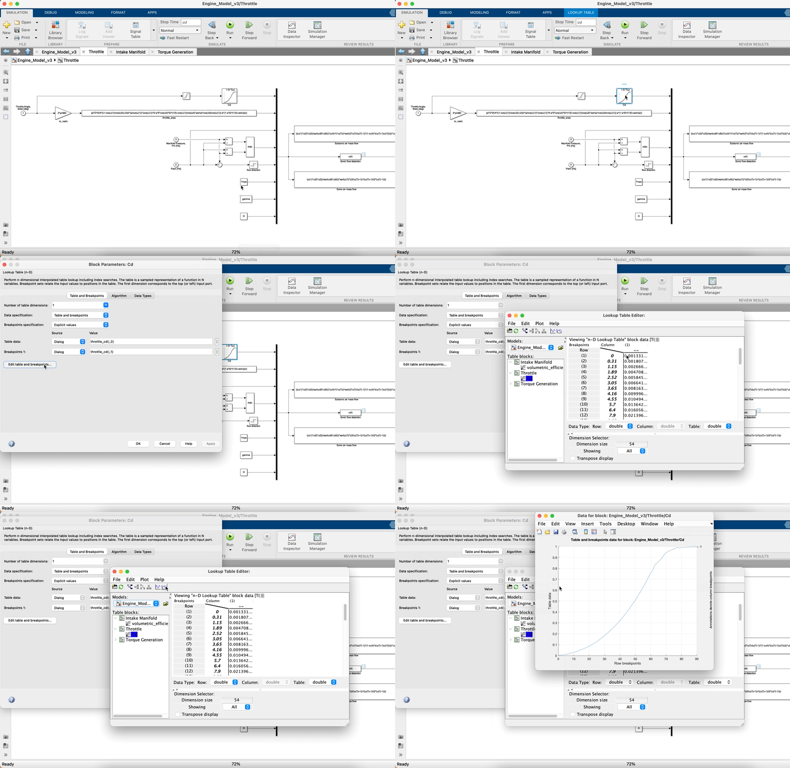
Use a 1-D lookup table block to evaluate $C_d$ as a function of throttle angle (note the units), the data for $C_d$ is available within the parameter file. When you are doing this have a look at the structure of the data and you will see that the first column is the opening angle in degrees, the second column is $C_d$. The table breakpoints are therefore the first column of the matrix and the table data i.e. the value that is output (as a function of the opening angle input) is the discharge coefficient. If you would like to check that you have entered the parameters correctly then click on Edit table data and breakpoints in the lookup table parameters as shown below.

The above method can also be used to view and check the others tables, including n-D tables, used elsewhere in this lab.
Intake Manifold
Open the Intake Manifold block, again note the inputs and outputs to the block. Using the equations in the lecture slides create the block structure to calculate Manifold Pressure and Air Mass Flow to the cylinder. The way to do this is to implement the speed-density equation to calculate the mass flow out of the manifold.
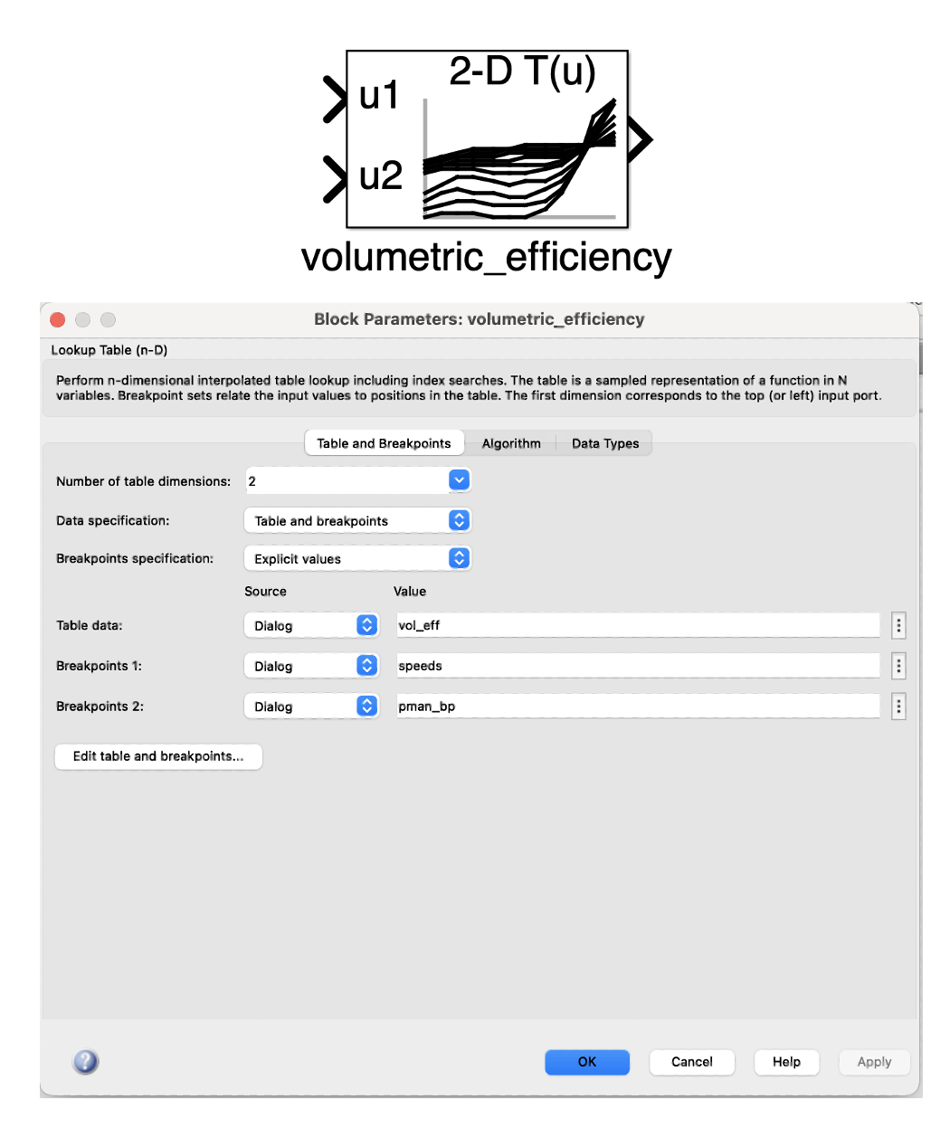
\[\dot{m}_{out}=\eta \frac{P_{\text {man }}}{R T_{\text {man }}} \frac{V_{\text {disp }}}{120} N_{\text {eng }} \nonumber\]Remember to multiply the speed-density equation by the volumetric efficiency, this will need to be included in the model using a 2D lookup table as follows;

To calculate the manifold pressure you will need to take the difference between the mass flow coming into the manifold this gives a $ \frac{dm}{dt} $ in the manifold from which a $ \frac{dP}{dt} $ can be calculated by using the ideal gas equation;
\[\frac{dP}{dt} = \frac{dm}{dt}\frac{RT}{V} \nonumber\]Integrating this you will get manifold pressure, $ P_{man}$. This can then be fed back to calculate volumetric efficiency which you will need to calculate the volumetric efficiency which is used to calculate the mass flow out of the manifold. Note that this is a circular calculation, the algebraic loop is broken by the integrator (which will need an initial condition setting).
Torque Generation
Open the Torque Generation submodel. Using the equation given for friction torque (noting the units) and the data provided for the torque as a function of engine speed and air mass flow use a 2D lookup table to evaluate torque. Recorded torque measurements are available in the parameters file.
As an extension to this try to fit a simple polynomial model to the data and use instead an equation to evaluate torque based on the inputs (this is easy using the curve fitting, cftool in Matlab). Try and evaluate any differences in the polynomial model and the data as represented (and interpolated) by the 2D lookup table.
Obtaining Results
Simulating
In the simulation configuration parameters change the solver to ode5 (Dormand-Prince) fixed step solver with a step size of no greater than 0.0001 seconds (note that such a small step is required because this is a stiff system).
Run the model for the first time at predefined engine speed and WOT, look at the data to see if your model outputs are sensible. If any errors are detected resolve these before continuing.
Analysis and plotting
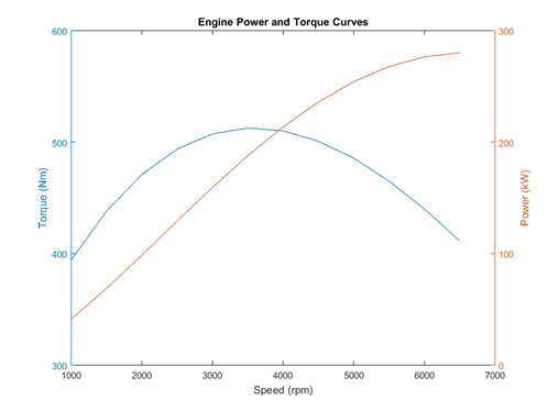
Run the model at a minimum of three speed points at WOT and record torque. Fit a cubic polynomial to the data using the Matlab polyfit() function and plot the curve at each of the speed points. On the same graph but using a different colour also plot the engine data obtained from the table below. Think about any differences there are between the two curves, why do these arise?
From the torque data (or by addition to your model) calculate the engine brake power. Plot this on a separate graph along with the engine recorded power data available in the table over the page.
Model Debugging
Once you have got your model running check the output torque at the model top level to ensure for the inputs shown in the figure below outputs match. Note that in the version of the model shown below in all of the lookup tables the default Algorithm settings have been changed (see the tab in the block properties). For a perfect match you will need to change the interpolation method to cubic spline, extrapolation to clip and the search method to linear search.

Figure: Engine model outputs for debugging
If your model doesn’t produce the outputs as shown above, try splitting the model into subsystems to locate the problem. For example, as shown below, you can isolate the throttle subsystem. Isolating the subsystem and providing fixed inputs should mean, for a correct subsystem, that the outputs are the same as that shown in the previous diagram. If they aren’t then there is something wrong in the isolated subsystem.

Figure: Isolating subsystems for debugging
In addition to the above, the data in the next section can help you assess if you model is correct over a range of speeds.
Additional Information

Engine Power and Torque
| Speed [rpm] | Torque [Nm] | Power [kW] |
|---|---|---|
| 1000 | 394.4 | 41.3 |
| 1500 | 438.1 | 68.8 |
| 2000 | 470.9 | 98.6 |
| 2500 | 493.8 | 129.3 |
| 3000 | 507.4 | 159.4 |
| 3500 | 512.6 | 187.9 |
| 4000 | 510.1 | 213.7 |
| 4500 | 500.8 | 236.0 |
| 5000 | 485.5 | 254.2 |
| 5500 | 465.0 | 267.8 |
| 6000 | 440.0 | 276.5 |
| 6500 | 411.7 | 280.1 |