Section 5: Ride Dynamics
Table of contents
These notes are an extremely condensed and reduced version of Chapter 5 from Thomas D. Gillespie’s Fundamentals of Vehicle Dynamics. It is well worth reading this chapter (and others) from the book. All the figures in this section come from the book.
The Ride System
The Excitation Sources are the inputs to the system as shown in Figure 1 below.
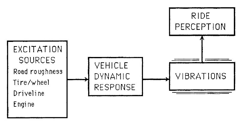
Figure 1: The ride system
These might be illustrated in the time domain, but are more often shown in the frequency domain (for example as a Power Spectral Density plot. The system reacts to these inputs, mapping them into Perceived Ride which might itself be shown in terms of a measurable output, such as vehicle body vertical acceleration.
Excitation: Road Roughness
The principal excitation source is the road. Figure 2 shows a PSD of three measured roads along with average frequency models for them.
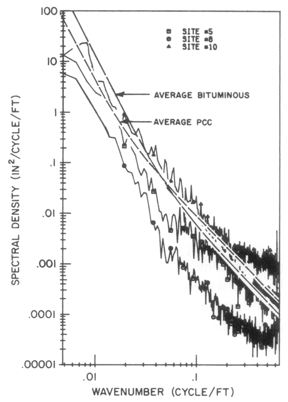
Figure 2: Typical spectral densities of road elevation profiles
The frequency model is;
\[G_{Z}(v)=\frac{G_{O}\left[1+\left(v_{O} / v\right)^{2}\right]}{2\pi v^{2}} \label{eq1}\]| $G_z(v)$ | PSD amplitude $(feet^2/cycle/foot)$ |
| $\nu$ | Wavenumber $(cycles/foot)$ |
| $G_0$ | Roughness magnitude parameter $(1.25\times10^5$ for rough roads, $1.25\times10^6$ for smooth roads) |
| $\nu_0$ | Cutoff wavenumber ($0.02 \space cycle/foot$ for rough roads, $0.05 \space cycles/foot$ for smooth roads |
The simple model of Equation \ref{eq1} can be used in combination with a random number sequence to generate test roads which are random in themselves, but yet have approximately representative frequency content. Multiplication of the original wavenumber (cycles per foot) by a known constant vehicle speed (feet per second) gives a more recognisable PSD;
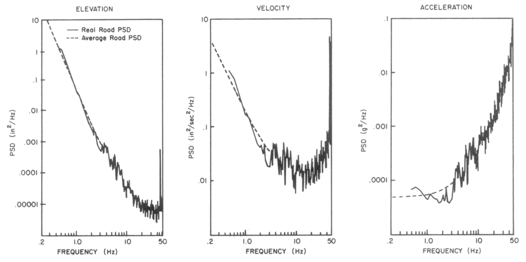
Figure 3: Elevation, velocity and acceleration PSD’s of road roughness input to a vehicle travelling at 50mph on a real and average road
Excitation: Secondary effects
Vibration from imperfection of the wheel or driveline, and from the engine, cause further excitations, usually at frequencies higher than the principal wheel-hop and body-bounce modes that we are most interested in. Note, Figure 4, illustrating wheel runout; although the tyre is complex, the model is just a collection of simple springs, we’ll see this is quite common in basic vehicle dynamic modelling.
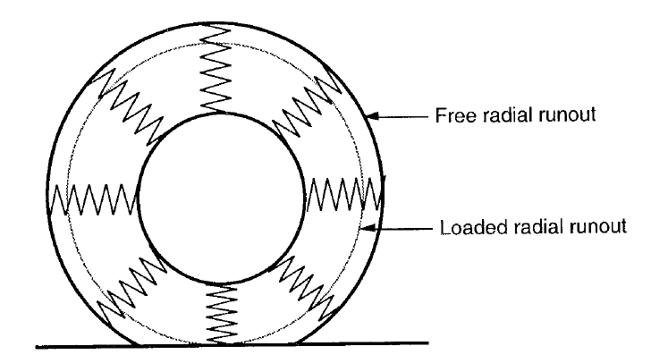
Figure 4: The radial spring model
Runout refers to the springs expanding and contracting, any unevenness causes an effect similar to wheel mass imbalance, giving a cyclical input at the frequency of the wheel rotation speed. Harmonics of the multiple spring model can also cause cyclical disturbance. Did you know tyres are sometimes square?
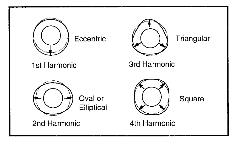
Figure 5: Radial nonuniformities in a tyre
The simplest Ride model: The Quarter Car
Although simple, the quarter car model is adequate and can be an accurate representation of real vehicle vertical motion. This is the first model that we will build and analyse on this course.
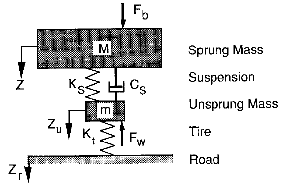
Figure 6: Quarter car model
Typical values of parameters for a large saloon;
| M | 300 kg |
| m | 30 kg |
| $K_s$ | 20000 N/m |
| $K_t$ | 160000 N/m |
| $C_s$ | 1500 Ns/m |
In order to perform some quick hand calculations on the expected frequencies and damping ratios given the parameter values, we can also think of the quarter car model in terms of modal simplifications.
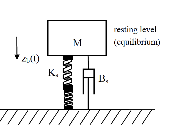
Figure 7: The quarter car model, body-bounce only
Firstly in the body-bounce variant, the unsprung mass is assumed zero, and the tyre and suspension springs are thus in series;
\[K_{b b}=\frac{K_{s} K_{t}}{K_{s}+K_{t}} \nonumber\]This gives a natural frequency for the body-bounce mode, in $[\mathrm{rad}/\mathrm{s}]$, of;
\[\omega_{n}=\sqrt{\frac{K_{b b}}{M}} \nonumber\]The actual (damped natural) frequency of vibration is affected by the damping ratio, $\zeta$;
\[\omega_{d}=\omega_{n} \sqrt{1-\zeta^{2}} \nonumber\]which is given according to the damping constant actually used ($B_s = C_s$);
\[\zeta=\frac{C_{s}}{\sqrt{4 K_{b b} M}} \nonumber\]Typically, a damping ratio of between 0.2 and 0.4 is achieved. What is the natural frequency, and damping ratio for the large saloon with parameter values given above?
REVEAL ANSWER
Natural Frequency, $\omega_n$;
\[K_{b b}=\frac{K_{s} K_{t}}{K_{s}+K_{t}} =\frac{20000 \times 160000}{20000+160000}=17777.78 N/m \nonumber\] \[\omega_{n}=\sqrt{K_{b b} / M} = \sqrt{17777.78 / 300} = 7.70 rad/s \nonumber\]Damping ratio, $\zeta$;
\[\zeta=\frac{C_{s}}{\sqrt{4 K_{b b} M}} = \frac{1500}{\sqrt{4\times17777.78\times300}} = 0.32\]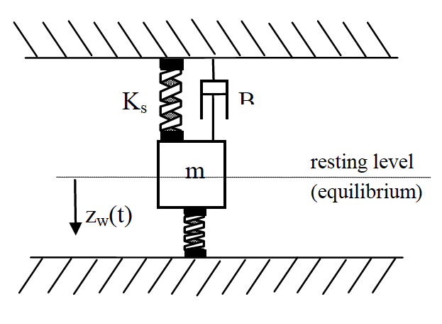
Figure 8: The quarter car model, wheel-hop only
WHAT IS WHEELHOP?
Looking at the wheel-hop only variant, here we assume that the sprung mass, $M$ hardly moves at all, so the unsprung mass, $m$ is governed by suspension and tyre springs in parallel;
\[K_{w h}=K_{s}+K_{t} \nonumber\]and;
\[\omega_{n}=\sqrt{\frac{K_{w h}}{m}} \nonumber\]in rad/s. Expected in the range 11 – 13 Hz, what is the wheel-hop frequency of the saloon car with parameter values given above?
REVEAL ANSWER
Wheel-hop Frequency, $\omega_n$;
\[K_{w h}=K_{s}+K_{t} = 20000+160000=180000\nonumber\] \[\omega_{n}=\sqrt{\frac{180000}{30}}=6000rad/s \nonumber\]Ride Response
Figure 9 illustrates, from left to right, input, model and output. The input and output here are the PSDs of road acceleration and vehicle acceleration respectively. The model shows the gain function (frequency response, or bode plot gain) between the two. Note how the road acceleration looks similar to that given in Figure 3 with high magnitudes at high frequencies. These high frequencies are not transmitted through the suspension, whose principal job is to isolate the vehicle body from undesirable inputs. In the model plot you can see the obvious body bounce resonance, around 1Hz and the kink around 10Hz showing the wheel hop resonance (we will see later, when looking at eigenstructure, that both modes of vibration affect both masses, at least to some extent). The output PSD shows how well the system has attenuated the high frequencies, whilst magnifying the response around 1Hz. You can look at the plots as input x model = output.
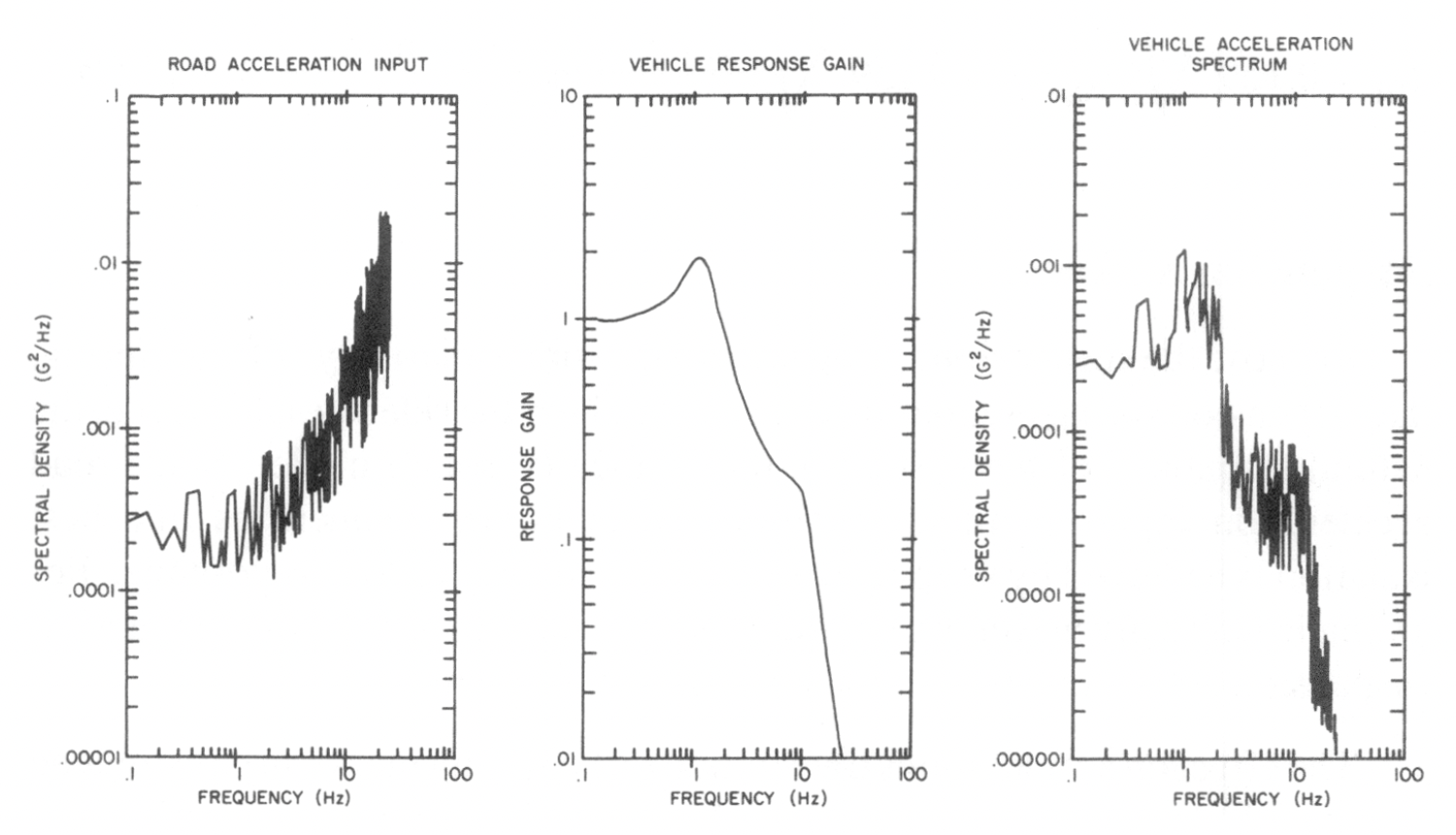 Figure 9: Isolation of road acceleration by a quarter car vehicle model
Suspension Stiffness and Damping
The magnitude of the body bounce peak is affected by what Gillespie refers to as the ride rate, $K_{bb}$ above. Because $K_s$ and $K_t$ act in series and $K_t$ is so much stiffer than $K_s$, $K_{bb}$ is dominated by $K_s$. In Figure 10 below, $K_s$ has been tuned to give a body bounce resonance frequency varying from 1Hz to 2Hz (without varying damping factor). This shows that as you increase the resonance frequency for body bounce, so the transmission of acceleration from the road to the vehicle will increase in magnitude by a large factor. The y-axis here is on a linear scale, so you can look at the area under the peak as a measure of the mean-square acceleration transmitted from road to vehicle. Obviously, the aim is to achieve good isolation, and reduce transmission, so lower $K_s$, and hence lower resonance frequencies are aimed for.
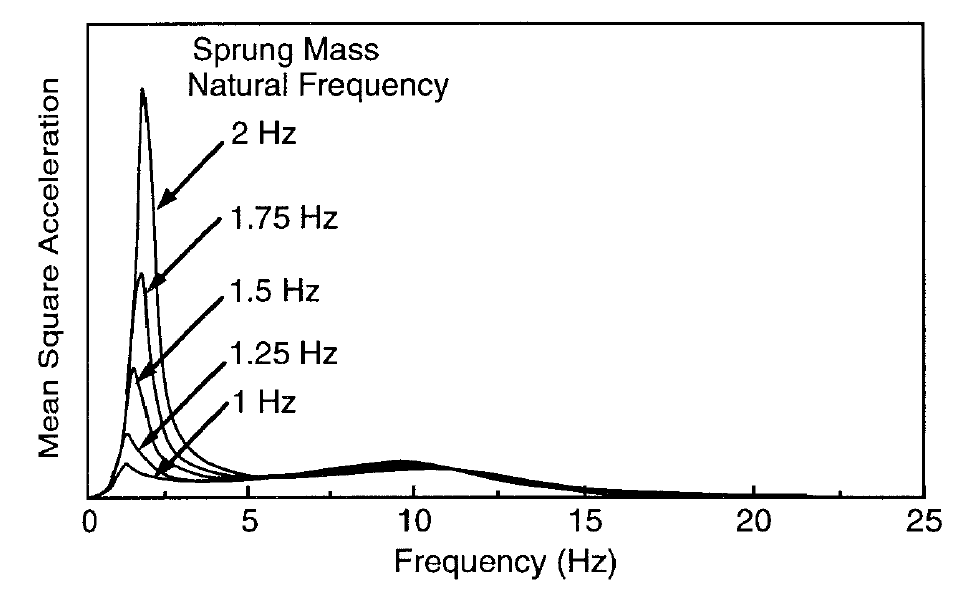
Figure 10: On road acceleration spectra with different sprung mass natural frequencies
The factors which prevent excessively low $K_s$ and hence lower ride rates are;
- Suspension travel – low spring rates necessitate greater suspension travel.
- Handling performance is affected by fluctuating vertical load on the tyre.
- Very low frequencies (well below 1Hz) would induce nausea (the points above restrict the frequency more than this).
Figure 10 isn’t totally honest however, as the damping in the suspension can always be increased, along with the suspension spring rate, to counter the high body bounce peak. The introduction of damping isn’t a simple solution though, because it reduces isolation at higher frequencies. Increases in damping essentially spread the range of frequencies through which vibrations are transmitted, whilst reducing the peak at a given (in this case body bounce) resonance;
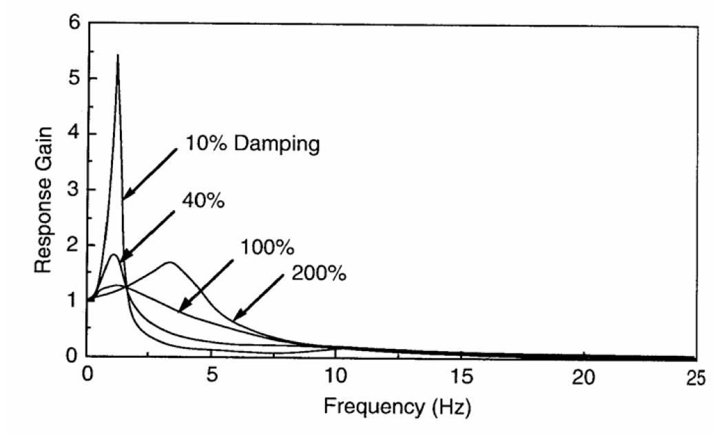
Figure 11: Effect of damping on suspension isolation behaviour
Figure 11 shows the effect of increasing $C_s$ to give damping ratio, $\zeta$ in the range 0.1 to 2. Note how at the extreme (200% damping) level, the stiff damper has effectively tied the body and wheel together, combining body bounce and wheel hop into one resonance at about 3.5Hz. This would be highly undesirable, due to its affect on the human body. Frequencies of 1Hz and 10Hz feel much better than 4Hz vertically.
Active Suspension
Although it is expensive to fit and run (in terms of fuel) controllable force generators (such as hydraulics, hydro-pneumatics), active suspension can, at least in theory, provide exceptional reductions in body bounce vibration transmission. Note that, interestingly, it is less easy to control the wheel hop peak.
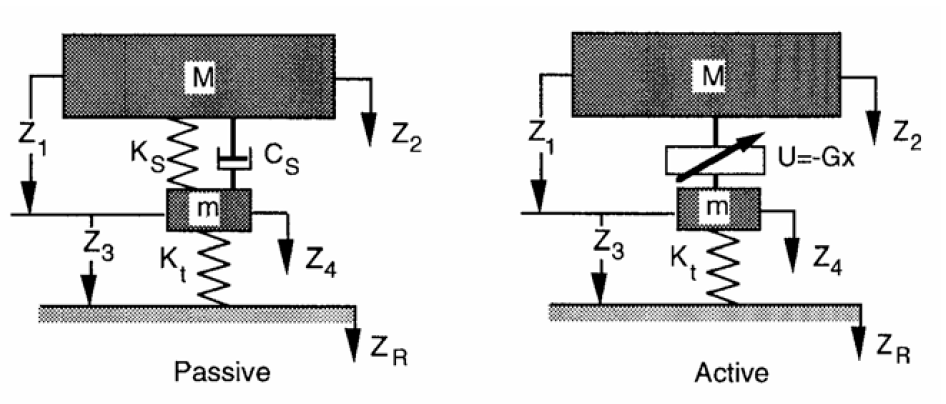
Figure 12: Quarter car model of active and passive suspension
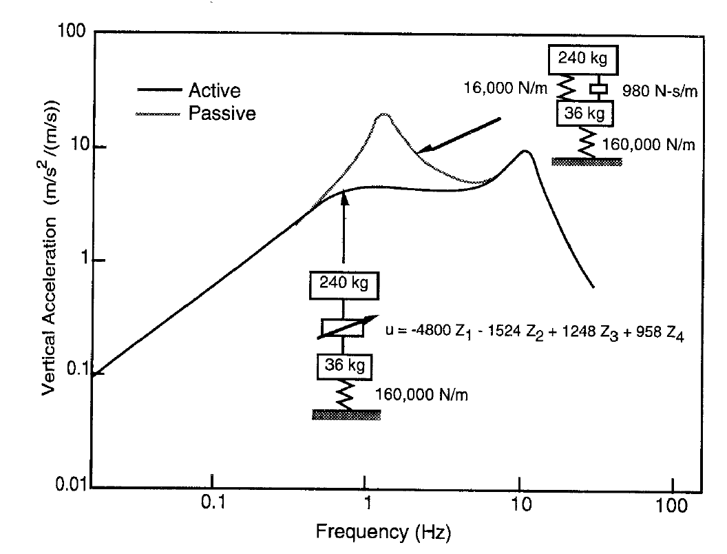
Figure 13: Comparison of vertical acceleration of active and passive systems
Bounce and pitch in combination
The quarter car model is good for investigating bounce only motion of the vehicle but more complex models are needed to give a more complete insight into why suspensions are designed the way they are. The natural progression is to include pitch motion, using the half-car model. Note that, although the analysis and discussion of this system gets more complicated, with front and rear suspensions being tuned to complement each other to give both desirable pitch and bounce, the model is not much more complicated. Figure 14 shows that we need only a rigid beam suspended on two springs to get a useful simulation model.
 Figure 14: Pitch plane model
We won’t get into the details of how the pitch and bounce modes behave, and how the ride rates of front and rear can be tuned here. It is worth noting a few basic issues though;
- Wheelbase filtering; Figure 15 shows how the spacing of the front and rear suspensions can couple with the wavelength in the road to give just bounce and just pitch. The effect is not really significant in practical terms (very few roads look like single sinusoids) but it is an effect worth understanding when it comes to interpreting PSDs or frequency responses from more complex systems.
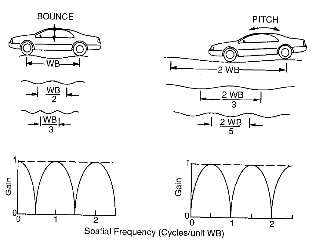
Figure 15: The wheelbase filtering mechanism - Position and direction of measurement; What you feel depends on where you are and in what direction you are interested and the type of motion. When we looked at the quarter car, we consider only vertical motion, but think about the simple beam of Figure 14 in pitch motion about its centre of gravity. If you sit at the centre, the rotation causes no motion. If you are above the centre of gravity the acceleration is fore-aft (not vertical) and only at the ends does pitch look mostly vertical. It is interesting to note that the principal problem associated with pitch is the fore-aft motion it produces for the passengers in spite of the much smaller moment arm.
- Lower ride rate at the front than the rear; A neat way of reducing the discomfort of pitching (pitch being worse than bounce, generally) is to make the front ride rate lower than the rear:
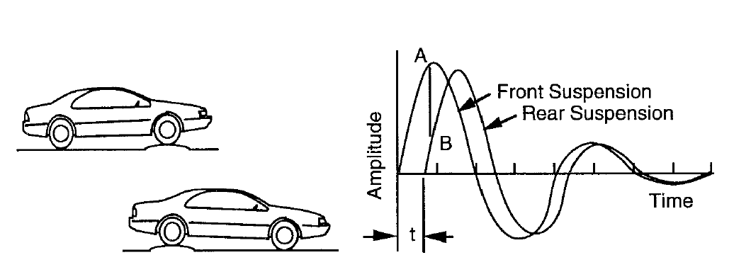
Figure 16: Oscillations of a vehicle passing over a road bump
With this design, as you meet a disturbance, you induce pitching instantaneously but with the rear suspension motion faster than the front, the motion resolves itself into bounce. Effectively, the rear oscillations catch up with those at the front, eliminating the phase lag that the constant delay in the wheelbase has caused.
Human Perception
We have looked at the PSD of ride (vertical) accelerations and the models of suspensions which give rise to these, across frequency. In order to complete the picture about how vehicles should be designed however, we also need to consider the dynamics of the human body. Vibrations start at the road, or in the vehicle and travel through the system of the vehicle (eg tyres, suspension) to the passenger compartment. From this point, the vibrations travel through the seat and passengers body before they are actually registered by the brain as uncomfortable. Thus we should consider the system of the body too.
One way of doing this is to subject people to vibration in an experiment and then get them to rate how uncomfortable each vibration is. In practice, this is done by testing one frequency at a time and building up a map of discomfort. The three plots below show lines of equal tolerance to various frequencies (x axis) applied at different amplitudes (y axis). The first two relate to vertical (ride) motion and the last one relates to fore-aft motion (pitch, and also shuffle).
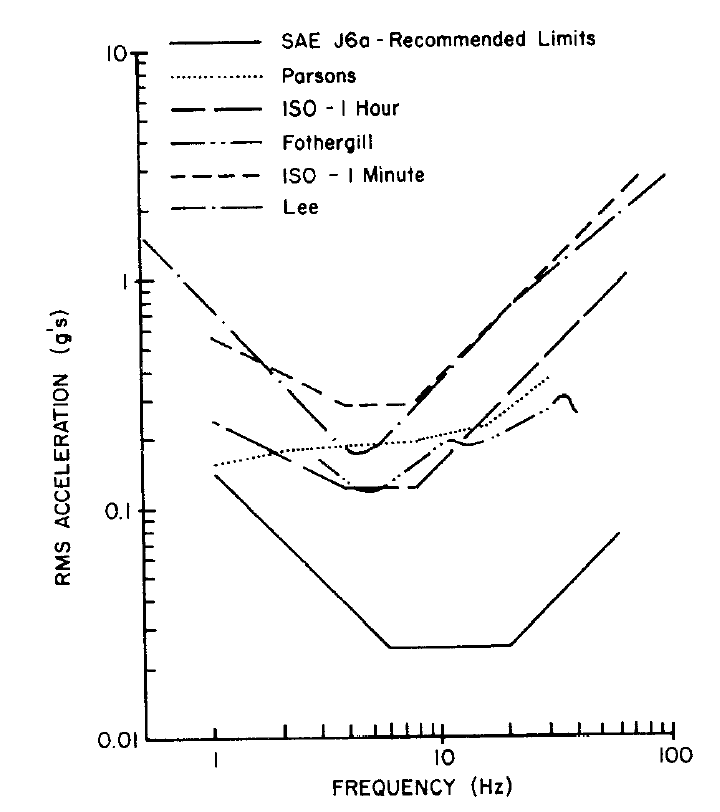
Figure 17: Human tolerance limits for vertical vibration
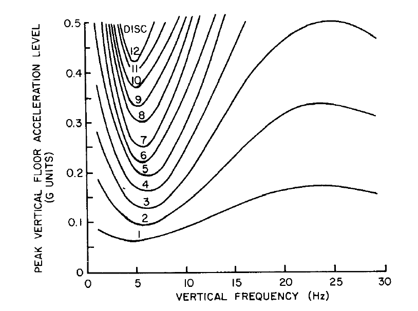
Figure 18: NASA discomfort for vibration in transport vehicles
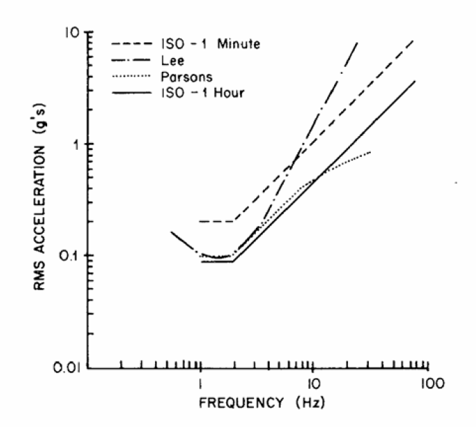
Figure 19: Human tolerance limits for fore/aft vibrations
A couple of summary conclusions:
- The NASA results correlate with vertical resonance frequencies of the organs of the human body in the abdominal cavity which lie in the range 4 – 8 Hz. This helps to explain why we have vehicle ride dynamics with resonance at 1Hz and 10Hz, (avoiding this range) and why the 200% damping solution in Figure 11 would be a disaster!
- Fore – aft tolerance is not the same as vertical tolerance. Fore-aft vibrations cause most concern at lower frequencies (1 – 2 Hz) and less concern as the frequency rises.