Section 2: Ordinary Differential Equations
Table of contents
What is an Ordinary Differential Equation and how does it relate to the real world?
We know about differentiation and integration in equations, for example;
\[\begin{gathered} y=3x^2+2\\ \frac{dy}{dx}=6x\\ \int{y}=x^3+2x+c \end{gathered} \nonumber\]These are what we call analytical functions, where the answer is itself an equation and you can plug in numerical values for $x$ to give the required value for $y$, $\frac{dy}{dx}$ or $\int{y}$. The dynamic behaviour of systems is related using differentiation and integration (with respect to time) but the relationships are more like;
\[M\frac{dv}{dt} = F - \frac{1}{2}\rho AC_{d}V^2 \nonumber\]Such that the derivative of the value depends on the value itself. This equation shows a good example, a simplified model of the longitudinal dynamics of a car. $F$ is the driving force at the wheels, and $v$ is the forward velocity. The second term on the right hand side represents aerodynamic losses, and $M$, $\rho$, $A$ and $C_d$ are (constant) parameters.
In dynamic simulation, because the dependent variable is time, $t$, we use the notation $\dot{v}$ in place of $\frac{dV}{dt}$. So velocity, $v=\dot{x}$ and acceleration, $a=\dot{v}=\ddot{x}$.
Although we can solve the equation analytically, the solution will only be valid for a fixed (input) force $F$, or if $F$ can be replaced by some other (analytical) function of time. In simulation, we want to generate time histories. To do this and allow for maximum flexibility in specifying $F$, we use numerical integration, rather than analytical solution.
NOTE: A variable is something which changes over time and which we could find a time history for. A parameter is a constant which is needed within the model but which might vary for separate simulation runs.
Generation of Differential Equations
Dynamic models are described in terms of a series of differential equations which can always be reduced to a set of first order differential equations. Two examples which we will refer to in these notes are the simplified single degree-of-freedom suspension model and the bouncing ball model. Note that the simplification stage of model design has already been completed for these cases, the former being reduced to a rigid mass suspended over a point which is fixed on the road by a simple spring and viscous damper (and which moves only vertically); the latter switches between contact and non-contact conditions.
Example 1: Body Bounce Suspension Model
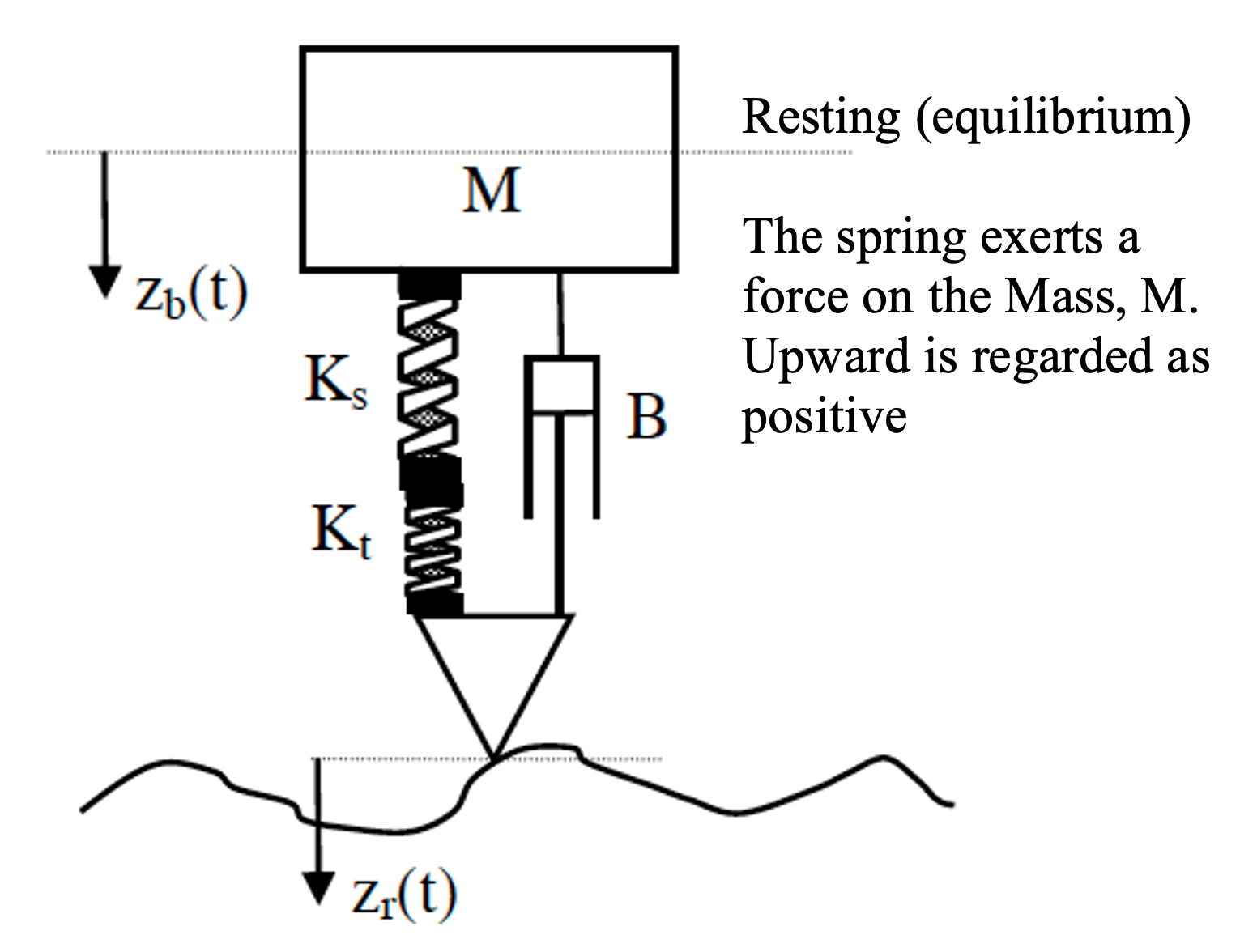
A simple body bounce model based on the schematic below can be created as follows.

Figure 1: Suspension (body bounce) model
Combining both of the springs to a single equivalent stiffness;
\[\frac{1}{K}=\frac{1}{K_{s}}+\frac{1}{K_{t}} \nonumber\]The force, $F_s$ is a combination of stiffness and damping terms;
\[F_{s}=K\left(z_{b}-z_{r}\right)+B_{s}\left(\dot{z}_{b}-\dot{z}_{r}\right) \nonumber\]and applying Newton’s law, $\sum F=m a$ to give;
\[-F_{s}=M \ddot{z}_{b} \nonumber\] \[M \ddot{z}_{b} = K\left(z_{r}-z_{b}\right)+B_{s}\left(\dot{z}_{r}-\dot{z}_{b}\right) \label{example_1:eq1}\]MORE ON SIGN CONVENTION
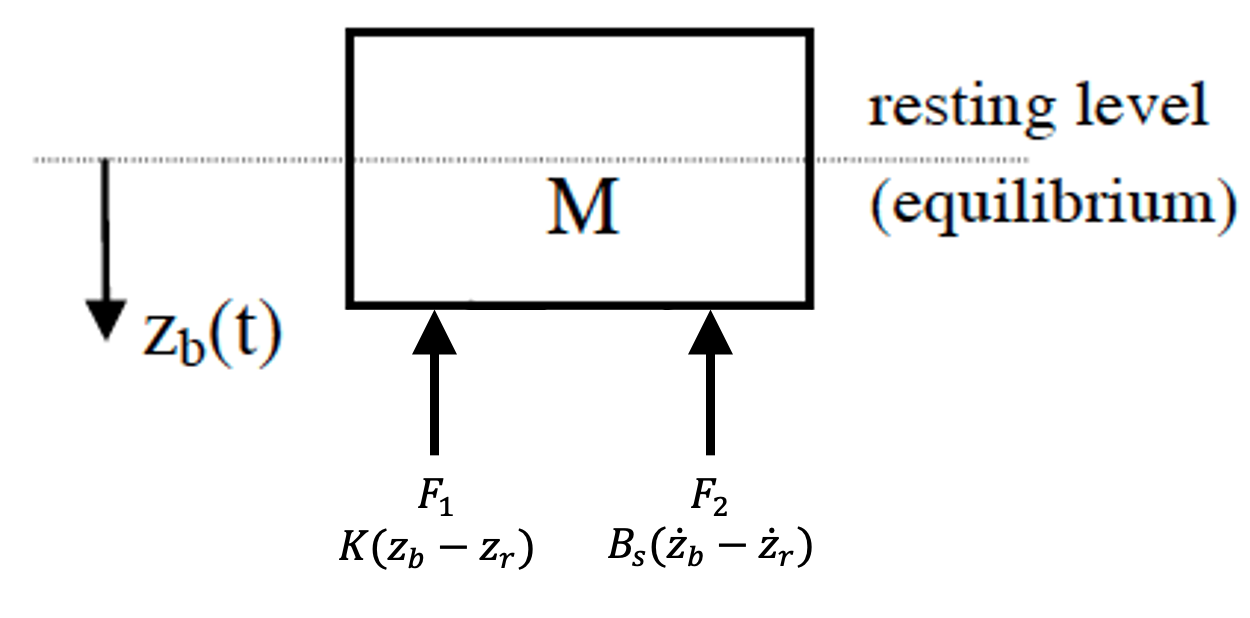
If you are struggling to understand how the above has been determined please look at the diagram below;

We imagine the forces from the spring, $F_1$ and damper, $F_2$ acting in the upward direction. Note that this is an arbitrary choice and we could have chosen another, e.g. both pointing down. With this choice the total force acting on the mass, $M$, will be described;
\[F_{s}=K\left(z_{b}-z_{r}\right)+B_{s}\left(\dot{z}_{b}-\dot{z}_{r}\right) \nonumber\]and since our forces act in the opposite direction to displacement, velocity and acceleration as defined by the arrow labelled $z_b(t)$ we say;
\[-\sum F=ma \nonumber\]and putting it all together we get the following (this is Equation \ref{example_1:eq1});
\[M \ddot{z}_{b} = K\left(z_{r}-z_{b}\right)+B_{s}\left(\dot{z}_{r}-\dot{z}_{b}\right) \nonumber\]If on the other hand we had chosen the opposite directions for $F_1$ and $F_2$ i.e. pointing downwards then $F_s$ would have looked like this;
\[F_{s}=K\left(z_{r}-z_{b}\right)+B_{s}\left(\dot{z}_{r}-\dot{z}_{b}\right) \nonumber\]and since forces act in the same direction as displacement, velocity and acceleration as defined by the arrow labelled $z_b(t)$ we say;
\[\sum F=ma \nonumber\]which leads to;
\[M \ddot{z}_{b} = K\left(z_{r}-z_{b}\right)+B_{s}\left(\dot{z}_{r}-\dot{z}_{b}\right) \nonumber\]which of course is the same as the previous one (Equation \ref{example_1:eq1})! Note that you won’t always end up with identical equations for different choices (of what is defined as positive or negative directions) but provided you have applied your choices consistently you will end up with the correct system equations.
For further information on this topic have a look at this video;
Now we reduce this single second order differential equation to a set of first order equations by defining system states, $x_1, x_2, x_3$, etc and inputs $u_1, u_2,…, u_n$ etc. We are trying to work out how to put the equations that describe the system dynamic behaviour in a form that looks something like this (remembering there are several other different forms we could use e.g. state space which we will look at later);
\[\begin{split} \dot{x}_1=f_1(\mathbf{x},\mathbf{u}) \\ \dot{x}_2=f_2(\mathbf{x},\mathbf{u}) \end{split} \label{example_1:eq2}\]Note that the notation $\mathbf{x}$ refers to the whole vector of several states i.e. $x_1, x_2, x_3, …, x_n$, etc whereas $x_1$ refers to just the one state. We could choose $x_1=z_b, x_2=\dot{z}_b, x_3=z_r$ and $u=\dot{z}_r$.
Writing Equation \ref{example_1:eq1} in terms of the states and inputs we get;
\[M\dot{x}_2=K(x_3-x_1)+B_s(u-x_2) \nonumber\]so the full set of equations in the form of Equation \ref{example_1:eq2} is;
\[\begin{split} &\dot{x}_1=x_2 \text{ (from the definition } x_1=z_b \text{)}\\ &\dot{x}_2=\frac{K}{M}(x_3-x_1)+\frac{B_s}{M}(u-x_2) \\ &\dot{x}_3=u \end{split} \label{example_1:eq2a}\]This is good but better yet is the choice of states, $x_1=z_r-z_b$, $x_2=\dot{z}_b$ and $u=\dot{z}_r$ because this removes the need for a third state. The model is then;
\[\begin{split} &\dot{x}_1=u-x_2 \\ &\dot{x}_2=\frac{K}{M}x_1+\frac{B_s}{M}(u-x_2) \end{split} \label{example_1:eq3}\]Example 2: Bouncing Ball Model Vertical Component Only
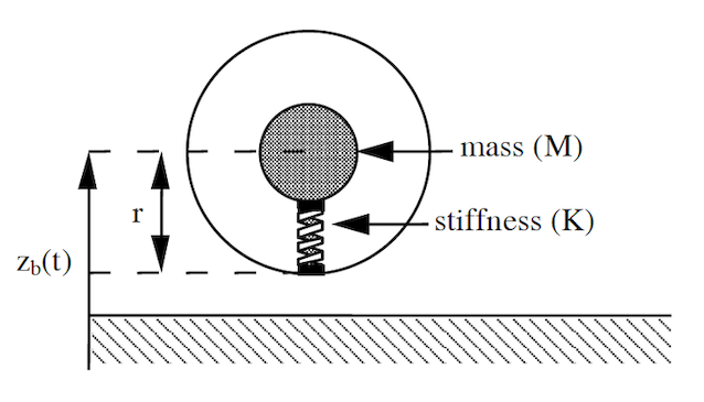
A simple bouncing ball model based on the schematic below can be created as follows.

Figure 2: Ball bounce model
When the ball is in contact with the ground this is very similar to the suspension, except that the road won’t move up and down and the reference is the ground, so the sign of positive $z_b$ is different.
The obvious state choice is $x_1=z_b$ and $x_2=\dot{z}_b$ and there is no input, $u$ here. The model is;
\[\begin{cases} {\dot{x}_1=x_2} & \text{if } x_1<r \\ \dot{x}_2=\frac{K}{M}\left(r-x_{1}\right)-\frac{B}{M} x_{2} &\\ {\dot{x}_1=x_2} & \text{otherwise}\\ \dot{x}_2=-g &\\ \end{cases}\]It’s interesting that we’re modelling mass, $M$ in the case if $z_b<r$ (in the $\frac{K}{M}$ and $\frac{B}{M}$ coefficients) but not modelling weight in this case. Compare with the otherwise case, where the acceleration is only due ot the weight (the $-g$ comes from $F=ma$ where the force is the ball weight).
In the ball model, there is no input ($u$) so we run different scenarios by setting different initial conditions, $x_1(0), x_2(0)$. In the suspension model we can also set initial conditions (and see how the suspension settles) and / or we can define a road input over time and play this into the model as it integrates. With the full set of information;
- Model
- Initial conditions, $\mathbf{x}(0)$
- Input(s) over time, $\mathbf{u}(t)$