Overview
Week 1
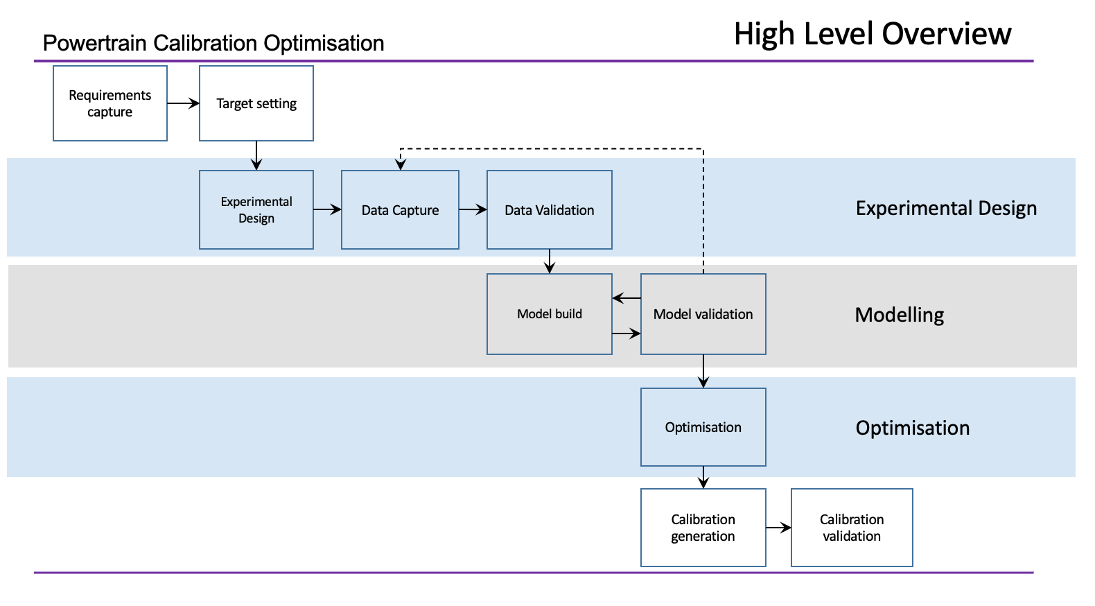
The first part of the lecture for this week introduces the module and the assessment structure. In the second part we will look at what calibration is.
As more technology is added to vehicles the complexity of the control system increases significantly. Powertrain controllers may have up to 50,000 parameters. Typically, up to 5000 of these may be changed to influence performance in terms of drivability, emissions and energy consumption. Calibration is the process by which information is obtained and decisions made to change parameter values to improve performance. In this first session we will be looking at, in overview, the various parts of the process and how these fit together to help engineers achieve optimal hardware performance. As we will see regardless of the powertrain technology, the process remains largely the same containing elements of optimisation, design of experiments, mathematical modelling and experimentation.
Week 1 Resources
| Lecture Slides |
| Introduction |
Week 2
At the core of the calibration process is the requirement to specify experiments, execute them to obtain data and create mathematical models based on this data. This could include emissions control systems, electric motors, engines, etc. These mathematical models are then used within a search algorithm or optimisation routine to find calibration parameter values that achieve best performance.
Underpinning all of the mathematical modelling is fundamental statistics that helps specify experiments, interpret results and create mathematical models. This week we will be looking at reviewing some fundamental statistical principles as we begin to consider these topics.
Week 2 Resources
| Lecture Slides |
| Statistics |
| Tutorial and Computer Labs |
| MATLAB Onramp |
| Simulink Onramp |
Week 3
The optimisation process is typically used to find actuator settings and controller gains that achieve the objectives of the calibration task. These may be, for example, minimum levels of noise or emissions. The model is used during optimisation as an inexpensive means of evaluating the consequence of changing actuator settings or controller gains on the outputs that relate to the calibration objectives. Without this systematic mathematical search, finding an acceptable solution for a high dimensional system would be almost impossible.
This week we will be looking at the fundamentals of the optimisation task to understand how we formulate the calibration task as an optimisation problem. This includes the lecture and a set of laboratory exercises completed this week and next. Later in the course, we will put this knowledge to use within a calibration exercise.
Week 3 Resources
| Lecture Slides |
| Optimisation |
| Computer Labs |
| Optimisation Laboratory |
Week 4
Models used within the calibration process (static or dynamic) require high levels of accuracy, due to this empirical models are used. These are built using a mathematical structure that is adjusted by comparing the model with data.
The collection of data in high dimensional systems is both expensive and time consuming. Design of experiments ensures that the experiments used for data collection are as efficient as possible collecting only the required data and no more.
This week we will look at the fundamentals of experimental design and how it can be deployed for use in data collection. Whilst the context in which we discuss this is powertrain calibration, experimental design methods, can be used wherever experimentation is undertaken. In fact it all started with a cup of tea.
Week 4 Resources
| Lecture Slides |
| Design of Experiments |
| Computer Labs |
| Design of Experiments |
Week 5
This week we will be looking at the topic of mathematical modelling in the context of powertrain calibration optimisation. There are a huge variety of different mathematical models that could be chosen from but not all of them would be able to represent the system in a form or to the level of accuracy required for the calibration task.
In the first part of the lecture we will be thinking about the different types of models, how they are grouped and what they are used for generally. Following this overview we will be investigating how they are fitted. The process of fitting is the one by which the coefficients (within the equations) are changed to ensure that the model output agrees with the data that has been collected during experiments.
There is no such thing as a perfect model! In the final part we will be looking at model performance evaluation and what the residuals can tell us about the model that we have fitted. Residuals are the differences observed between the model prediction (based on some inputs) and the experimental data collected.
In the subsequent laboratory session you will be putting all of this into practice.
Week 5 Resources
| Lecture Slides |
| Mathematical Modelling |
| Computer Labs |
| Modelling Principles |
Week 6
During this week we will be looking at the coursework briefs. This will provide an introduction to each and explain how the lectures and laboratories relate to each of the requirements. As a reminder due dates for each coursework is shown in the table below.
| Coursework | Due Date |
|---|---|
| MATLAB Onramp | 1 March 2022 |
| Planning Experiments | 3 May 2022 |
| Investigating Engine Emissions | 31 May 2022 |
Week 6 Resources
| Coursework Brief 2 |
| Planning Experiments |
| Coursework Brief 3 |
| Investigating Engine Emissions |
Week 7
This week we will begin the calibration exercises. These are a sequence of exercises to help you understand how each part of the calibration process fits with the other and of course have practice at undertaking the act of calibration yourself.
In addition we will be looking at the practice of engine testing within a research and development environment including a tour of an engine test facility. This is included to help you with your coursework and gain a better understanding of how complex the data collection task can be.
Week 7 Resources
| Introduction to the Calibration Exercise |
| Introduction to the Calibration Exercise |
| Engine Testing |
| Engine Testing |
Week 8
This week there is no lecture. The time allocated to the module is to be used for completing the calibration exercise.
Week 9
What does the future hold for calibration. In this weeks lecture we will be taking a look forward to try and understand how the calibration activity will evolve over the next five years. Instead of discussing particular technologies we review methods that will enable the calibrator to deal with a multitude of, as yet, unknown technologies.
Week 9 Resources
| Future Challenges |
| Future Challenges |