Acceleration Analysis (Vector Loop Method)
Four-Bar Linkage Vector Loop Equations
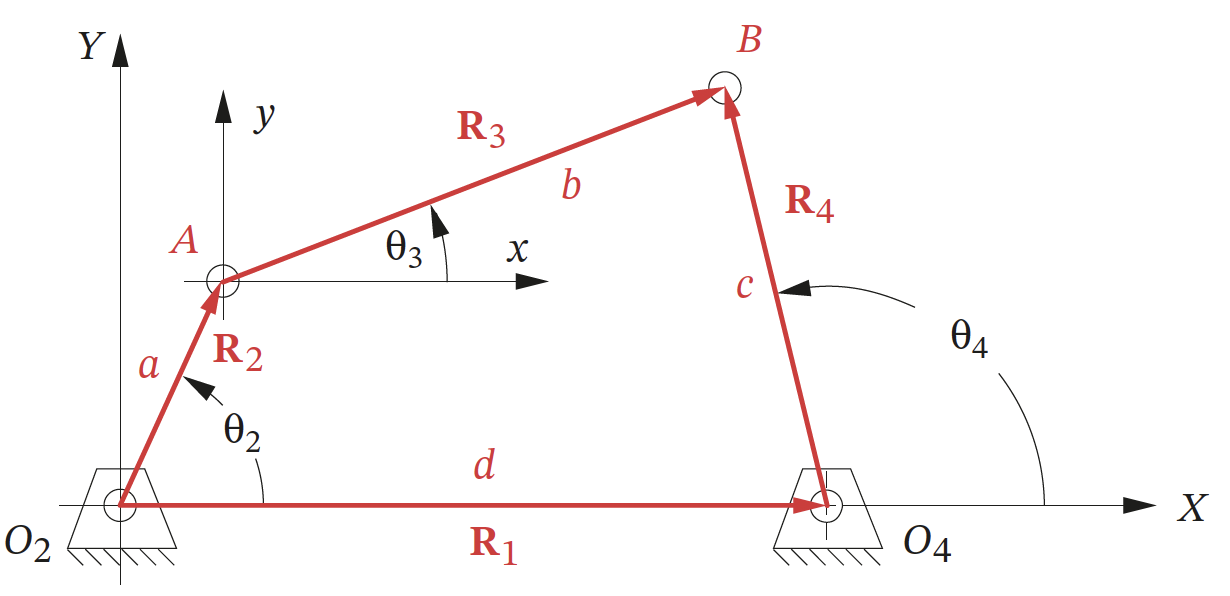
The derivation of the vector loop equation for a four-bar linkage mechanism involves defining the position vectors of the links and the angles between them. The four-bar linkage consists of four links connected by four joints, forming a closed loop as shown in the figure below.
Vector Loop Equation
The vector loop equation is derived by summing the position vectors around the closed loop of the four-bar linkage and setting their sum to zero:
\[\mathbf{R}_A+\mathbf{R}_{BA}-\mathbf{R}_{BO_4}-\mathbf{R}_{O_4}=0\]To obtain an alternative form of the equations, often used in analysis, complex number notation can be used for the position vectors. Using complex notation, the following is obtained
\[a e^{j\theta_2}+b e^{j\theta_3}-c e^{j\theta_4}-d e^{j\theta_1}=0\]where $a$, $b$, $c$ and $d$ represent the scalar length of each of the links.
Euler’s equation, $e^{j\theta} = (\cos \theta + j \sin \theta)$ may also be substituted into the equations to obtain this form
\[a(\cos\theta_2+j\sin\theta_2)+b(\cos\theta_3+j\sin\theta_3)-c(\cos\theta_4+j\sin\theta_4)-d(\cos\theta_1+j\sin\theta_1)=0\]Solving for Accelerations
Determining accelerations from the vector loop equation follows the same structure as the position and velocity analyses.
Previously, in Velocity Analysis we differentiated the position loop
\[a e^{j\theta_2} + b e^{j\theta_3} - c e^{j\theta_4} - d e^{j\theta_1} = 0.\]Because the ground link is fixed, $\theta_1$ is constant and its time derivatives are zero. The differentiated velocity loop is therefore
\[j a \omega_2 e^{j\theta_2}+j b \omega_3 e^{j\theta_3}-j c \omega_4 e^{j\theta_4}=0.\]Differentiating once more with respect to time gives
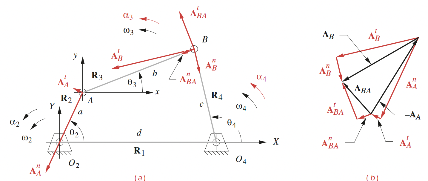
\[\left(j a \alpha_2 e^{j\theta_2}-a \omega_2^2 e^{j\theta_2}\right) +\left(j b \alpha_3 e^{j\theta_3}-b \omega_3^2 e^{j\theta_3}\right) -\left(j c \alpha_4 e^{j\theta_4}-c \omega_4^2 e^{j\theta_4}\right)=0.\]This equation contains both tangential terms proportional to $\alpha$ and normal terms proportional to $\omega^2$. In vector form, it is the acceleration loop
\[\mathbf{A}_A+\mathbf{A}_{BA}-\mathbf{A}_B=0.\]where
\(\mathbf{A}_A=\left(\mathbf{A}_A^t+\mathbf{A}_A^n\right)=\left(j a \alpha_2 e^{j\theta_2}-a\omega_2^2 e^{j\theta_2}\right),\) \(\mathbf{A}_{BA}=\left(\mathbf{A}_{BA}^t+\mathbf{A}_{BA}^n\right)=\left(j b \alpha_3 e^{j\theta_3}-b\omega_3^2 e^{j\theta_3}\right),\) \(\mathbf{A}_B=\left(\mathbf{A}_B^t+\mathbf{A}_B^n\right)=\left(j c \alpha_4 e^{j\theta_4}-c\omega_4^2 e^{j\theta_4}\right).\)
Similarly to the process in Velocity Analysis, substitute $e^{j\theta}=\cos\theta+j\sin\theta$ to give
\[\begin{aligned} &\left[a \alpha_2 j\left(\cos\theta_2+j\sin\theta_2\right)-a \omega_2^2\left(\cos\theta_2+j\sin\theta_2\right)\right] \\ &\quad+\left[b \alpha_3 j\left(\cos\theta_3+j\sin\theta_3\right)-b \omega_3^2\left(\cos\theta_3+j\sin\theta_3\right)\right] \\ &\quad-\left[c \alpha_4 j\left(\cos\theta_4+j\sin\theta_4\right)-c \omega_4^2\left(\cos\theta_4+j\sin\theta_4\right)\right]=0 \end{aligned}\]which simplifies to
\[\begin{aligned} &\left[a \alpha_2\left(-\sin\theta_2+j\cos\theta_2\right)-a \omega_2^2\left(\cos\theta_2+j\sin\theta_2\right)\right] \\ &\quad+\left[b \alpha_3\left(-\sin\theta_3+j\cos\theta_3\right)-b \omega_3^2\left(\cos\theta_3+j\sin\theta_3\right)\right] \\ &\quad-\left[c \alpha_4\left(-\sin\theta_4+j\cos\theta_4\right)-c \omega_4^2\left(\cos\theta_4+j\sin\theta_4\right)\right]=0 \end{aligned}\]Collecting the terms into real and imaginary components gives, first, the real part:
\[-a \alpha_2 \sin \theta_2-a \omega_2^2 \cos \theta_2-b \alpha_3 \sin \theta_3-b \omega_3^2 \cos \theta_3+c \alpha_4 \sin \theta_4+c \omega_4^2 \cos \theta_4=0,\]and then the imaginary part:
\[a \alpha_2 \cos \theta_2-a \omega_2^2 \sin \theta_2+b \alpha_3 \cos \theta_3-b \omega_3^2 \sin \theta_3-c \alpha_4 \cos \theta_4+c \omega_4^2 \sin \theta_4=0.\]These two equations are solved simultaneously for $\alpha_3$ and $\alpha_4$:
\[\begin{aligned} \alpha_3 & =\frac{(a \alpha_2 \sin \theta_2 + a \omega_2^2 \cos \theta_2 + b \omega_3^2 \cos \theta_3 - c \omega_4^2 \cos \theta_4) (c \cos \theta_4)}{(c \sin \theta_4)(b \cos \theta_3)-(b \sin \theta_3)(c \cos \theta_4)} \\ & \quad - \frac{(c \sin \theta_4)(a \alpha_2 \cos \theta_2 - a \omega_2^2 \sin \theta_2 - b \omega_3^2 \sin \theta_3 + c \omega_4^2 \sin \theta_4)}{(c \sin \theta_4)(b \cos \theta_3)-(b \sin \theta_3)(c \cos \theta_4)} \\ \alpha_4 & =\frac{(a \alpha_2 \sin \theta_2 + a \omega_2^2 \cos \theta_2 + b \omega_3^2 \cos \theta_3 - c \omega_4^2 \cos \theta_4)(b \cos \theta_3)}{(c \sin \theta_4)(b \cos \theta_3)-(b \sin \theta_3)(c \cos \theta_4)} \\ & \quad - \frac{(b \sin \theta_3)(a \alpha_2 \cos \theta_2-a \omega_2^2 \sin \theta_2-b \omega_3^2 \sin \theta_3+c \omega_4^2 \sin \theta_4)}{(c \sin \theta_4)(b \cos \theta_3)-(b \sin \theta_3)(c \cos \theta_4)} \end{aligned}\]Having calculated $\alpha_3$ and $\alpha_4$, the linear accelerations $\mathbf{A}_{A}$, $\mathbf{A}_{BA}$, and $\mathbf{A}_{B}$ can be determined directly from the complex rigid-body acceleration expressions.
\[\begin{aligned} \mathbf{A}_A & =a \alpha_2\left(-\sin \theta_2+j \cos \theta_2\right)-a \omega_2^2\left(\cos \theta_2+j \sin \theta_2\right) \\ \mathbf{A}_{BA} & =b \alpha_3\left(-\sin \theta_3+j \cos \theta_3\right)-b \omega_3^2\left(\cos \theta_3+j \sin \theta_3\right) \\ \mathbf{A}_B & =c \alpha_4\left(-\sin \theta_4+j \cos \theta_4\right)-c \omega_4^2\left(\cos \theta_4+j \sin \theta_4\right) \end{aligned}\]