Lecture 1: Analysis of Mechanisms

[For Illustration Only]

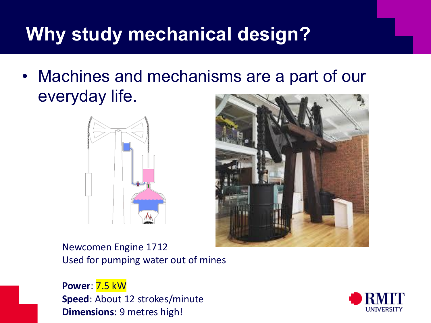
Mechanical design concerns machines that convert, transmit and control motion. Designers must consider force, speed, size and durability. Even early engines had large moving parts, repeated loads and useful power output. The basic questions of mechanism analysis have therefore been important for a long time.

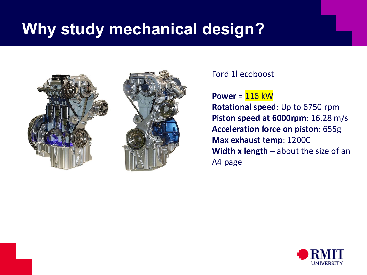
Modern engines show the difficulty of producing high power in a small space. High rotational speeds, high piston accelerations, high temperatures and limited space all act together. Links, joints, bearings, shafts and supporting structures must therefore provide both good performance and a long operating life.

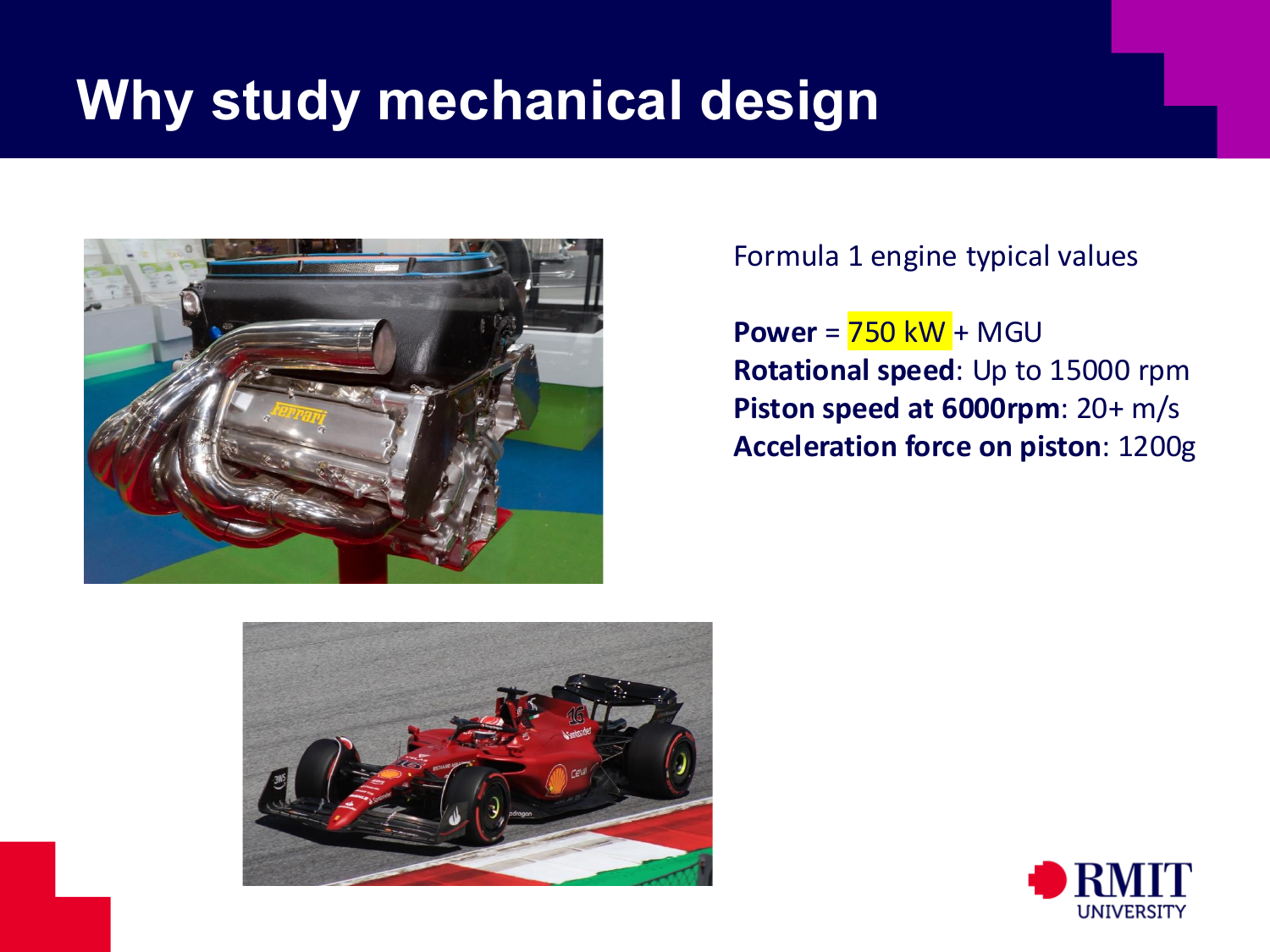
In high-performance machines, mechanism geometry and inertia become even more important. Very high speed and acceleration produce large dynamic loads. Small changes in geometry can therefore strongly affect stress, vibration, efficiency and service life.

Mechanical design is not limited to engines. The same ideas apply to vehicles, robots, aerospace equipment, consumer products, pumps, compressors and other machines. In each case, motion must be created, controlled, transmitted or used to operate a device.

The main topics are degree of freedom, types of motion, links and joints, kinematic diagrams and mobility calculations. These ideas help describe planar mechanisms, simplify real machines for analysis and determine whether an assembly can move as intended.

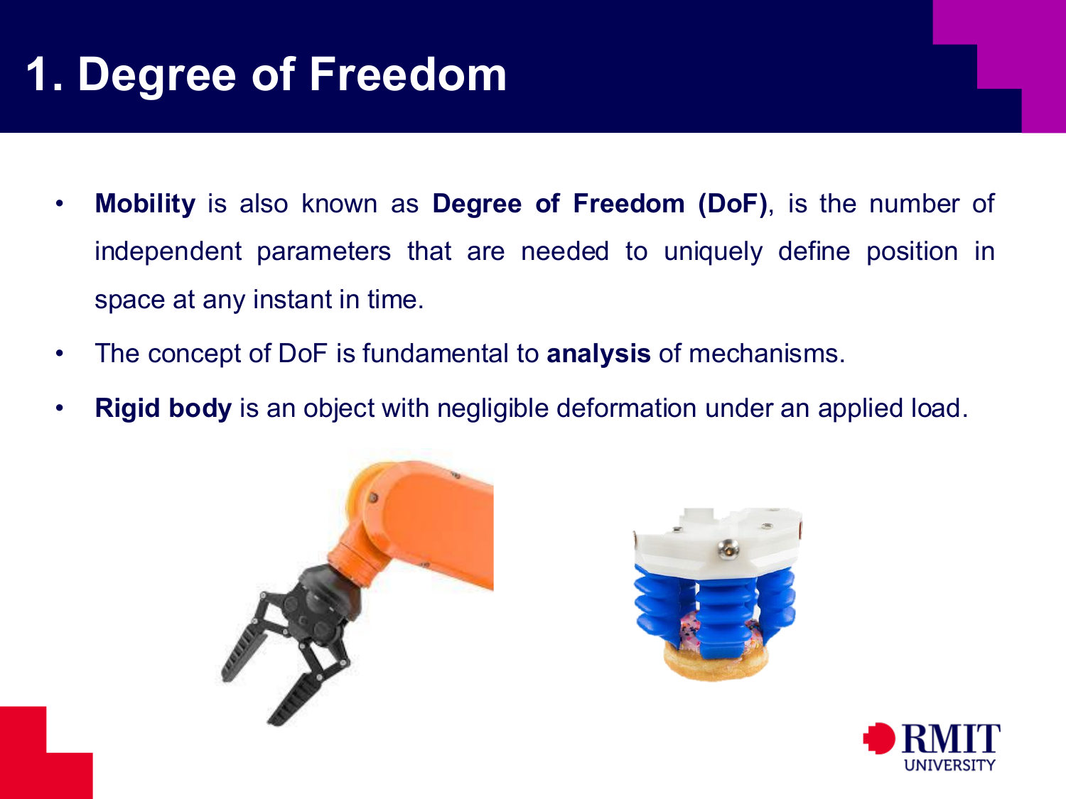
Mobility, or degree of freedom, is the number of independent values needed to define the position of a body or mechanism at one instant. It can also mean the number of independent inputs needed to produce a known motion.

This definition uses the rigid-body assumption. It ignores deformation, so motion can be described using geometry and constraints. When links are treated as rigid, the main question is how joints and supports prevent possible motions.

A system with one degree of freedom has one input variable that determines its position. Systems with more degrees of freedom need more independent coordinates to describe their motion fully.

Independent motions must be separate. If one coordinate can be calculated from another because of a joint or support, it is not an additional degree of freedom.

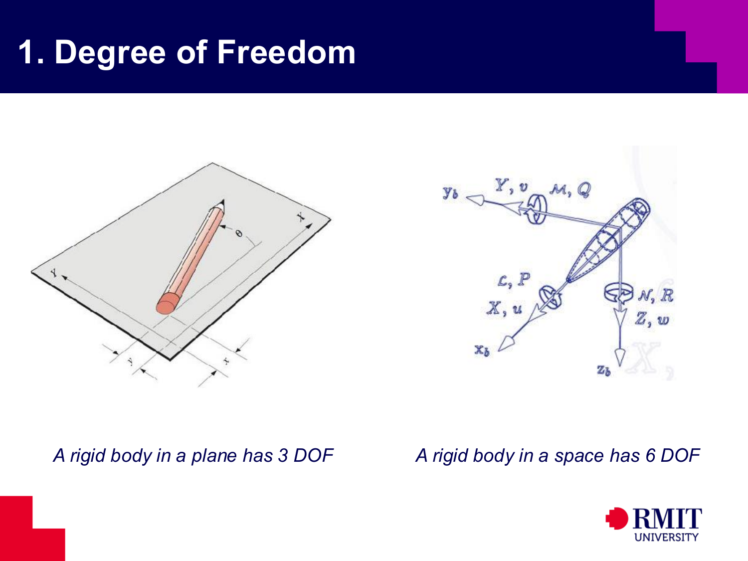
A rigid body in a plane has $3$ degrees of freedom: two translations and one rotation. A rigid body in space has $6$: three translations and three rotations. For a planar body, these are motion in $x$, motion in $y$ and rotation through an angle $\theta$.

Most examples are planar, so their mobility calculations use the planar case. Every unconstrained planar link begins with three possible motions. Joints and the ground then remove some of them.

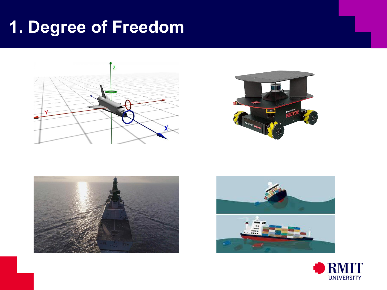
Real systems often combine translation and rotation. Their constraints determine which motions are possible. A vehicle moving on a plane, a ship that can roll and pitch, and a body moving freely in three dimensions all have different possible motions.

Constraints, not only the shape of a body, determine its possible motion. The same rigid body can have different degrees of freedom when it is free, guided in a slot, pinned to the ground or touching another body.

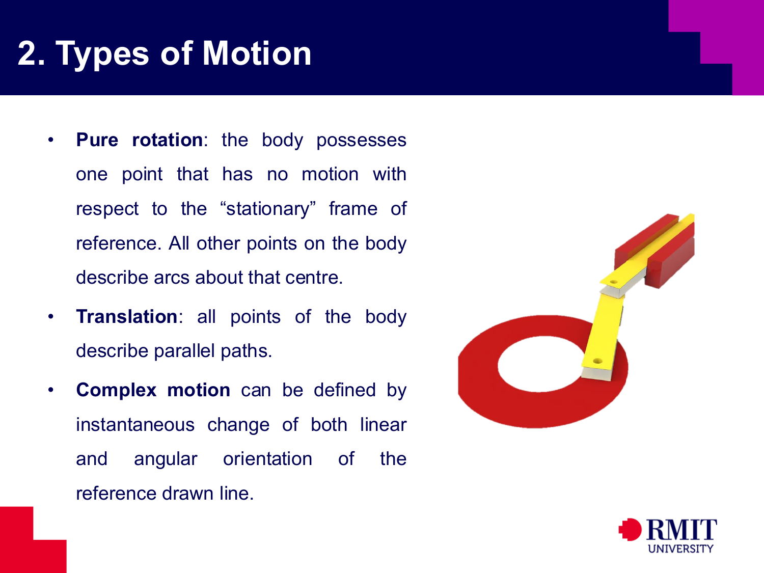
Planar rigid-body motion can be pure rotation, translation or general motion. In pure rotation, one point remains fixed and all other points move in circular paths around it. In translation, all points move along parallel paths. The body changes position but not orientation.

General motion combines translation and rotation, so position and orientation change together. Coupler links usually have this type of motion. It can be analysed using rigid-body principles after identifying the fixed points, moving links and joint constraints.

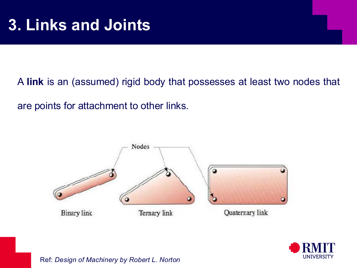
A link is a rigid body with at least two nodes where it can connect to other links. A node is a possible connection point. The number of nodes therefore determines how many connections a link can have.

Links are classified by their number of nodes. Binary links have two nodes, ternary links have three and quaternary links have four. Link order is important because it determines the number of connections and joints.

A joint connects two or more links and allows possible motion between them. A joint is also called a kinematic pair. Mechanism analysis focuses on the motion allowed or prevented by the connection, rather than the detailed shape of its parts.

A joint is defined by the relative motions that remain possible after the links are connected.

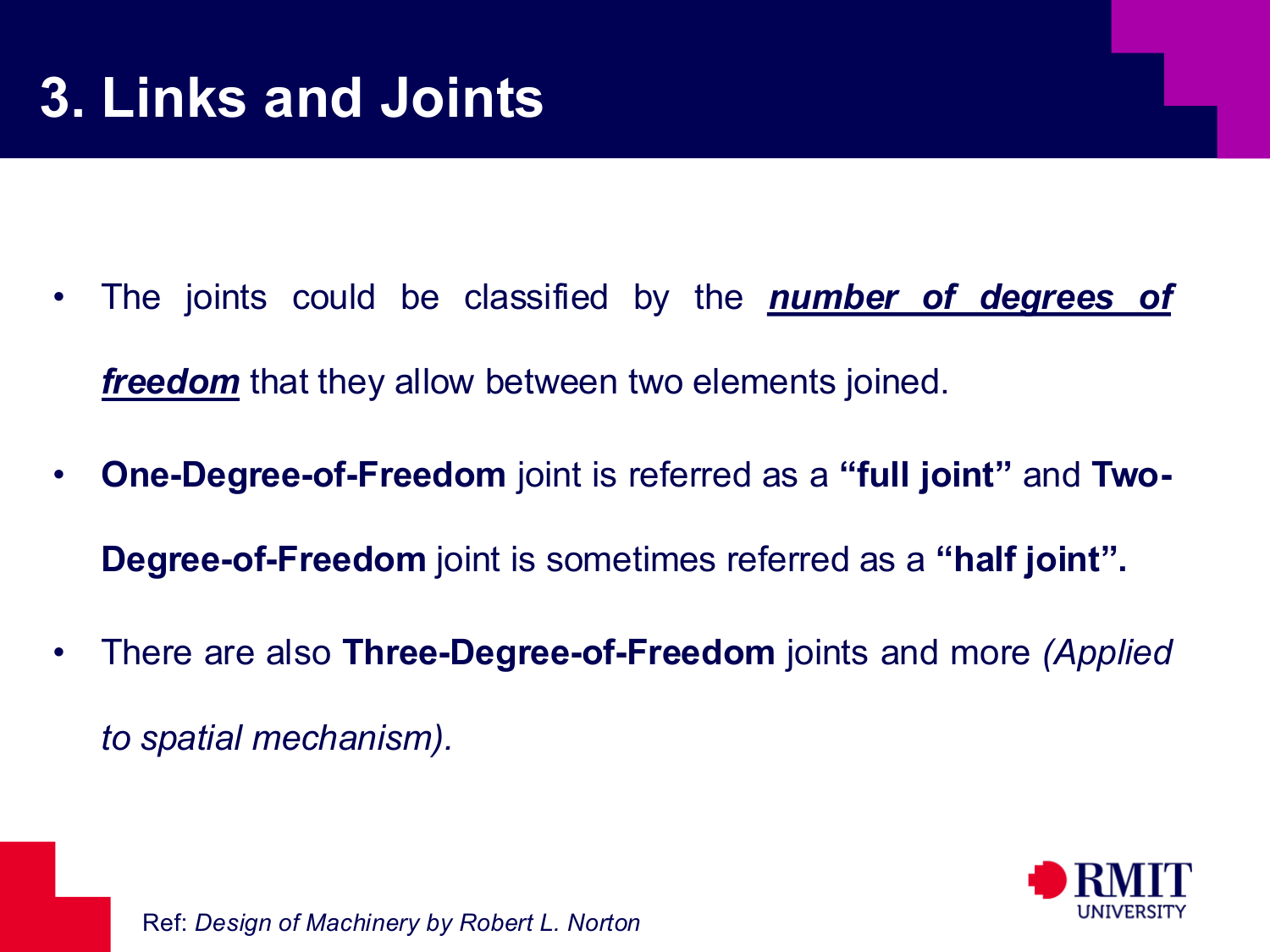
Joints may be classified by the number of degrees of freedom they permit between the connected links. In planar mechanism theory, a one-degree-of-freedom joint is often called a full joint, while a two-degree-of-freedom joint is called a half joint.

A full joint removes two relative motions between planar links, while a half joint removes only one. This difference is the reason the two joint types appear with different coefficients in mobility equations.

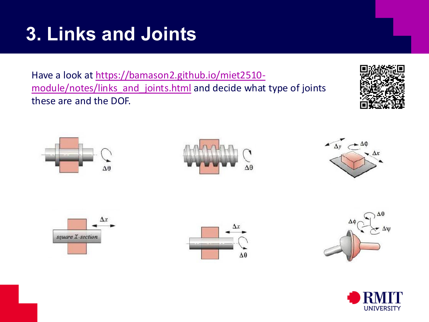
Different joint shapes allow different combinations of translation and rotation. A revolute joint allows rotation about one axis. A prismatic joint allows linear motion along one axis. Cylindrical, helical, planar and spherical joints allow other combinations of motion.

A pin-in-slot is a useful example because it leaves both sliding and relative rotation available, so it has two relative degrees of freedom. A simple pin joint leaves only rotation, and a slider leaves only translation.

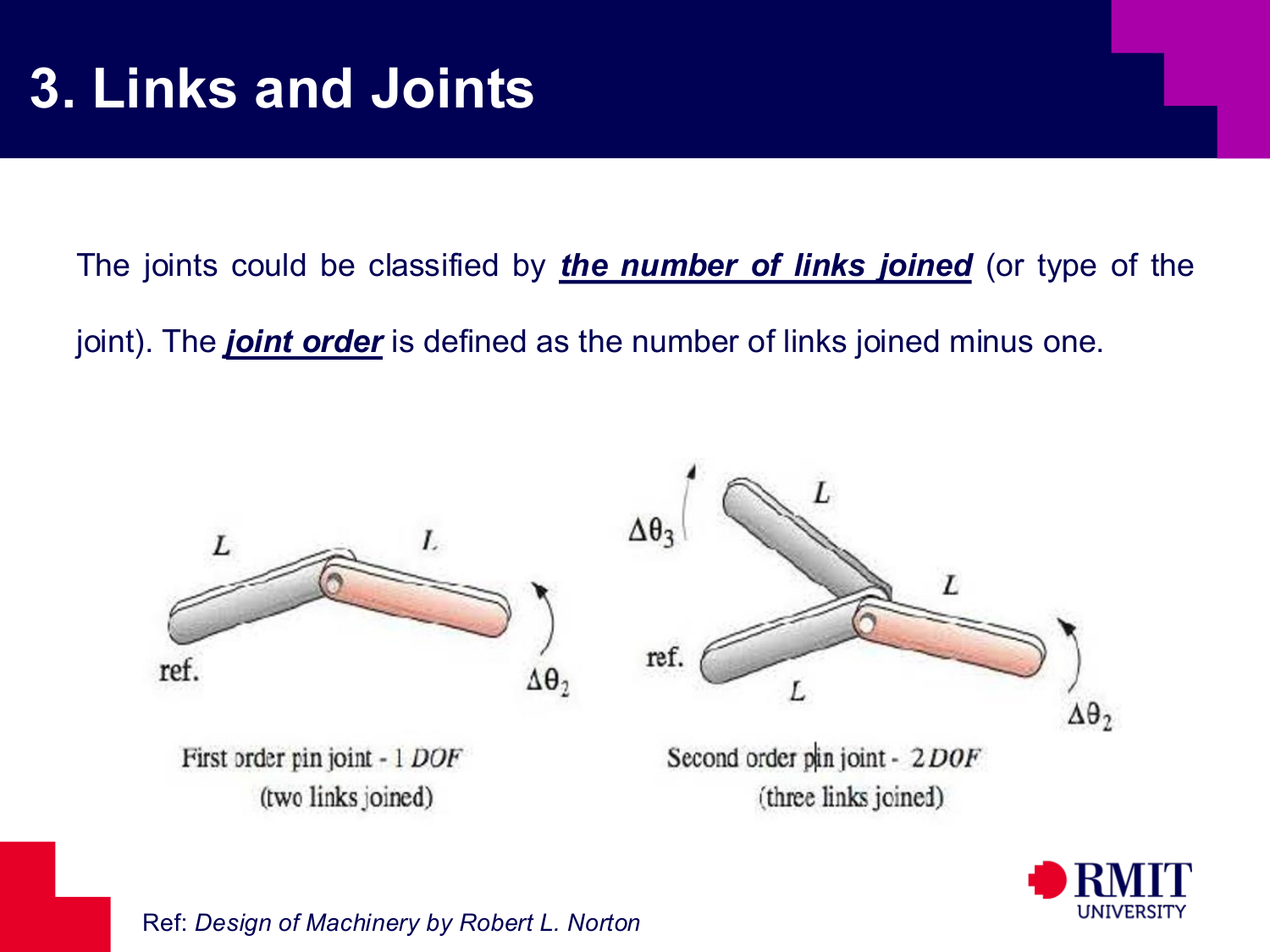
Joint order equals the number of connected links minus one. This distinguishes a normal two-link joint from a multiple joint, where three or more links meet at one location.

When counting joints, a pin joining three links is not one ordinary pin joint. It is counted as two first-order joints that share one centre. Multiple joints must therefore be shown carefully in the kinematic diagram.

More generally, if $n$ links meet at one joint centre, the connection contributes the equivalent of $n-1$ first-order joints. This is a counting rule, not a statement that there are physically separate pins.

A mechanism transmits motion in a planned way. A machine transmits both motion and energy to perform useful work. Some assemblies are analysed mainly for their motion. Others must also be checked for power, force transmission and work output.

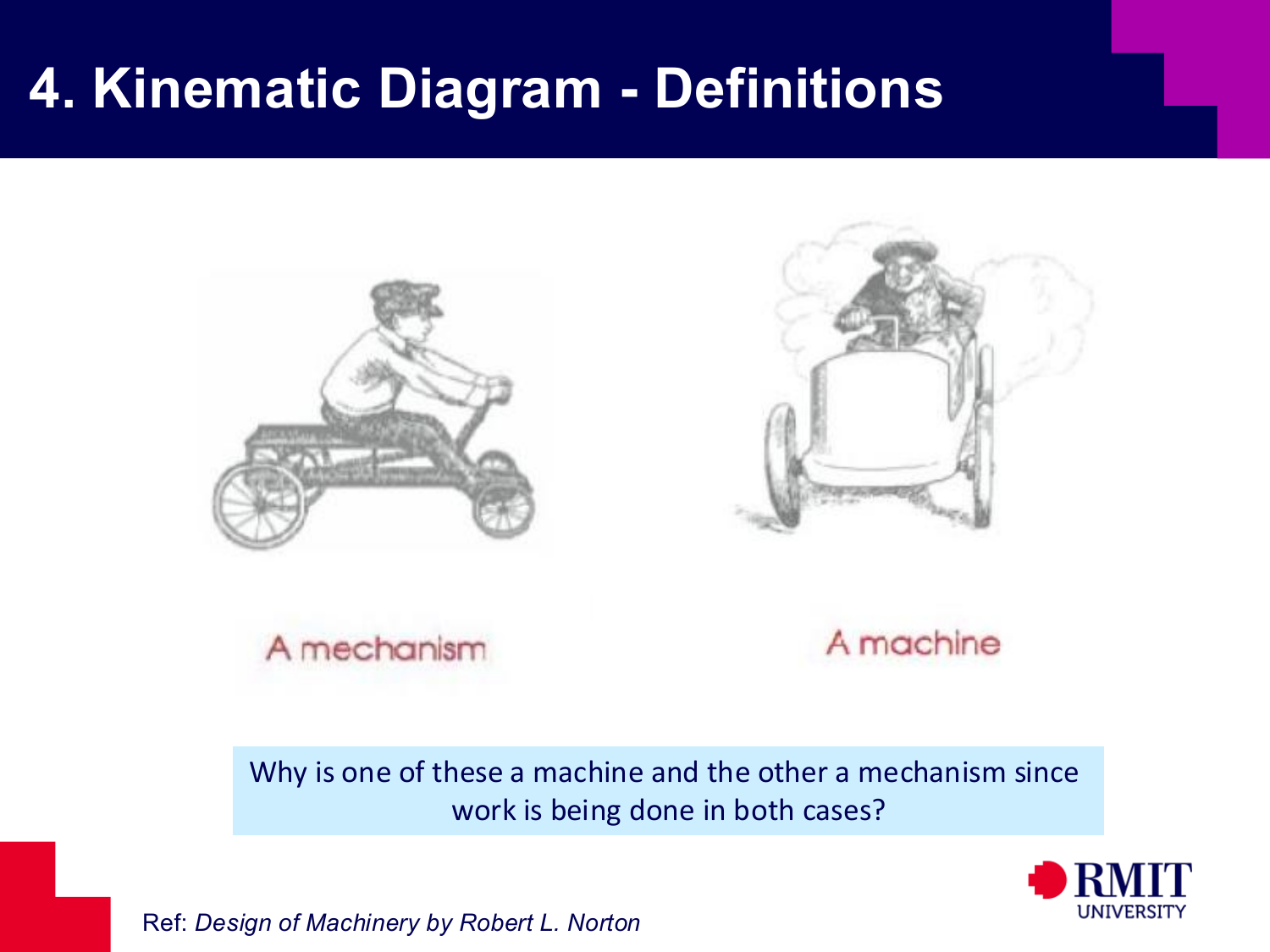
A mechanism and a machine may look similar because both can contain links and joints. The classification depends on their purpose. A mechanism mainly changes motion, while a machine also transfers energy and performs useful work.

The same linkage can therefore be studied in two ways. Kinematic analysis examines how motion is controlled and transmitted. Machine analysis also examines forces, torque, power and actuator input.

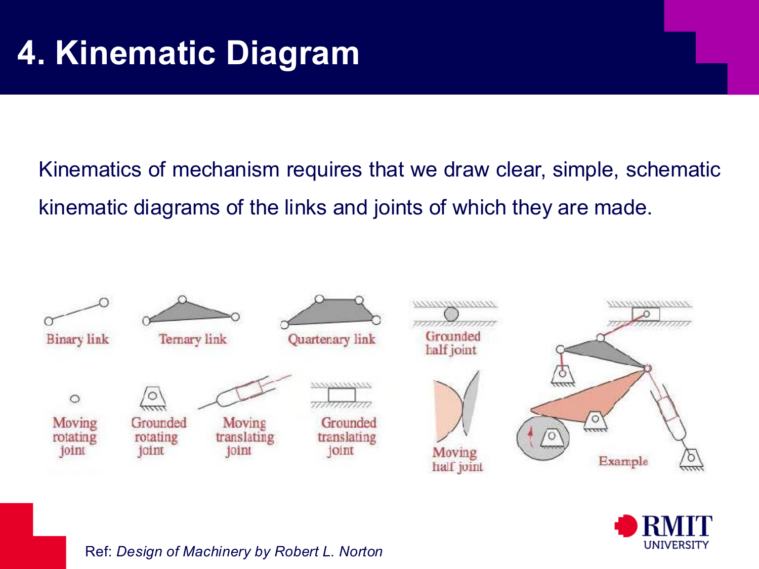
Kinematic analysis begins with a simplified diagram of the machine’s links and joints. A good kinematic diagram removes unnecessary details but keeps the connections, joint types and relative motions that control the mechanism.

The shape in a kinematic diagram may differ from the real part. It is chosen to show motion and connections clearly, not to copy the manufactured shape.

Fasteners, covers, decorative parts, and other features that do not affect the kinematic constraint structure are normally omitted. What remains is only the set of rigid bodies and joints that determine motion.

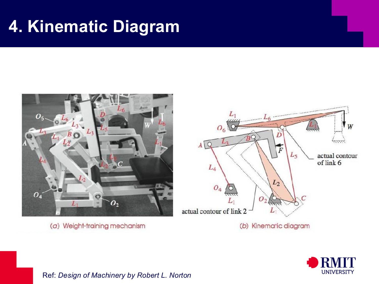
A complex device is easier to analyse after reducing it to its kinematic structure. The important features are the ground link, moving links, pivot locations and force application points. The full shape of the product is not needed after these features are identified.

The simplified diagram often places all links in one plane. Real parts may be at different depths, but their motion can still be treated as planar if the joints limit motion to one effective plane.

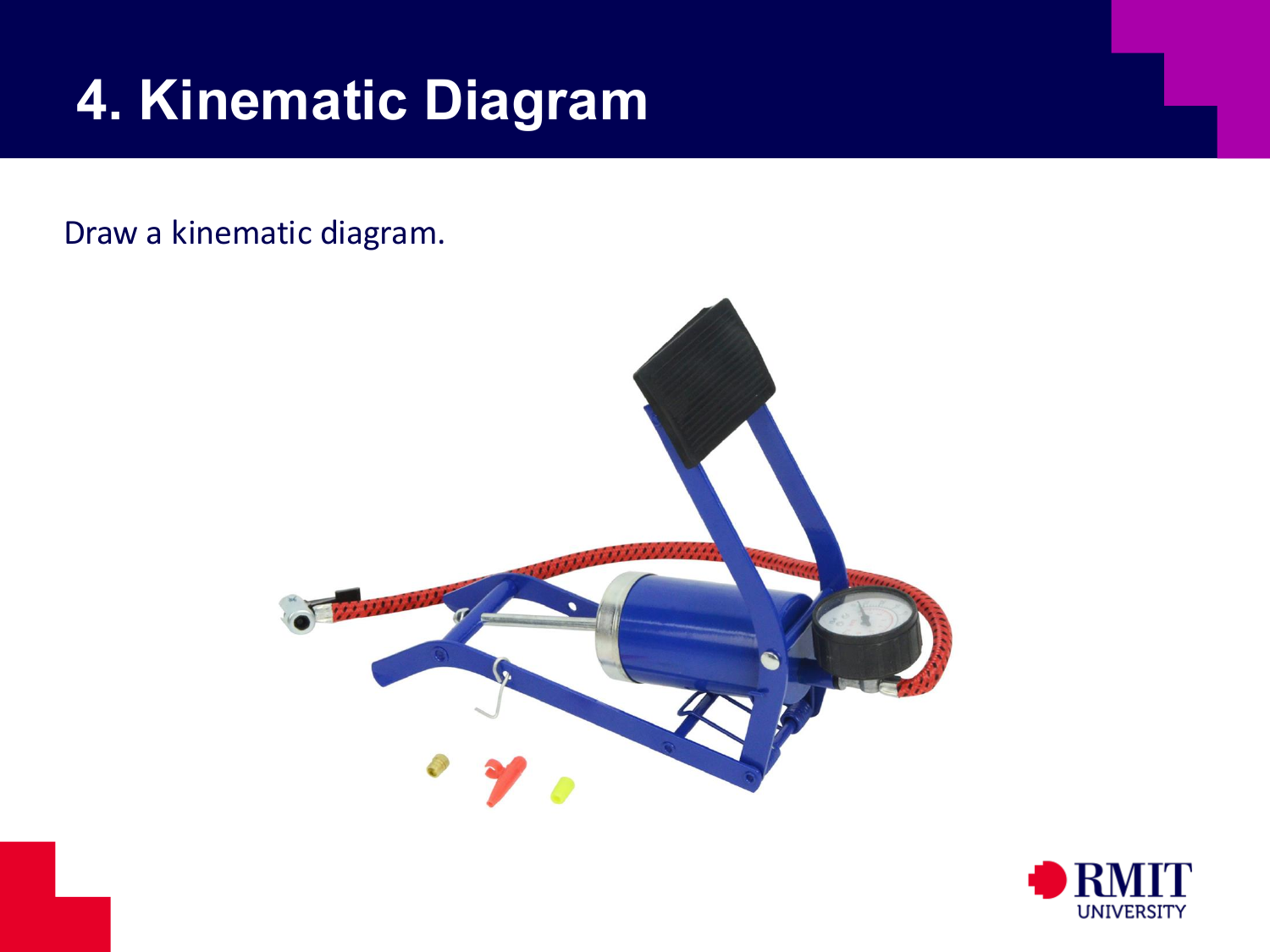
To draw a kinematic diagram, identify the ground link, moving links, joint types and the path from input motion to output motion. In a foot-operated pump, a linkage changes pedal motion into the back-and-forth motion of the pumping element.

An incorrect diagram produces an incorrect mobility count. Number each link clearly and mark shared joints because the calculation uses the simplified model, not the appearance of the product.

A practical method is to identify the fixed frame first, then mark each distinct moving rigid body once, and only then classify the joints between them. This reduces the risk of double-counting parts that belong to the same rigid link.

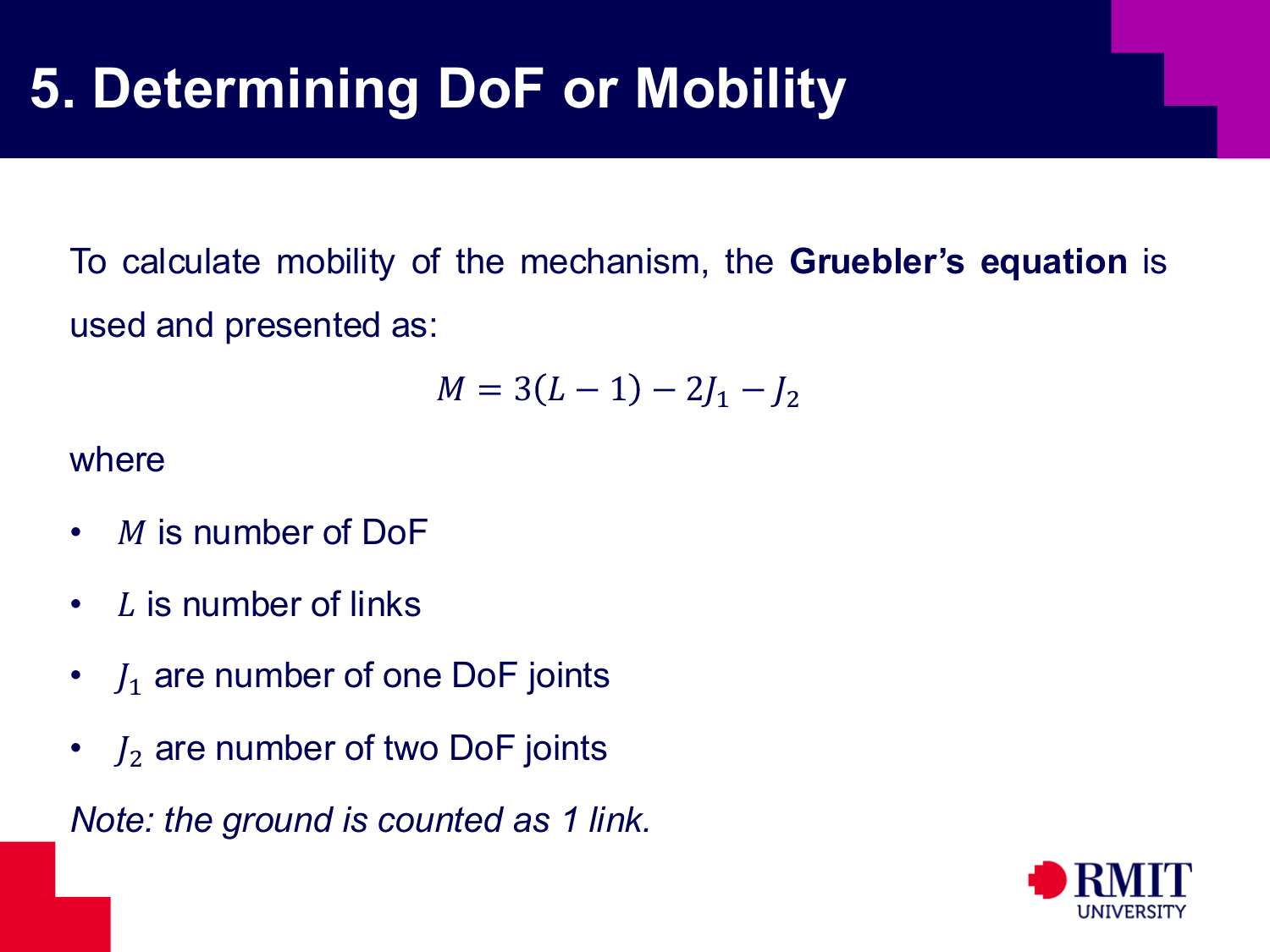
Mobility is calculated using Gruebler’s equation for planar mechanisms, \(M = 3(L - 1) - 2J_1 - J_2,\) where $M$ is the degree of freedom, $L$ is the number of links, $J_1$ is the number of one-degree-of-freedom joints, and $J_2$ is the number of two-degree-of-freedom joints. The ground is counted as one link, so the fixed frame or base must be included in the link count.

Each planar link starts with $3$ possible motions. The equation then subtracts the motions removed by joints and the ground. A full joint removes two relative motions, a half joint removes one, and fixing one link removes all three of that link’s motions.

When $M=1$, one input determines the position of the whole mechanism. When $M>1$, more than one independent input or coordinate is needed to define its position.

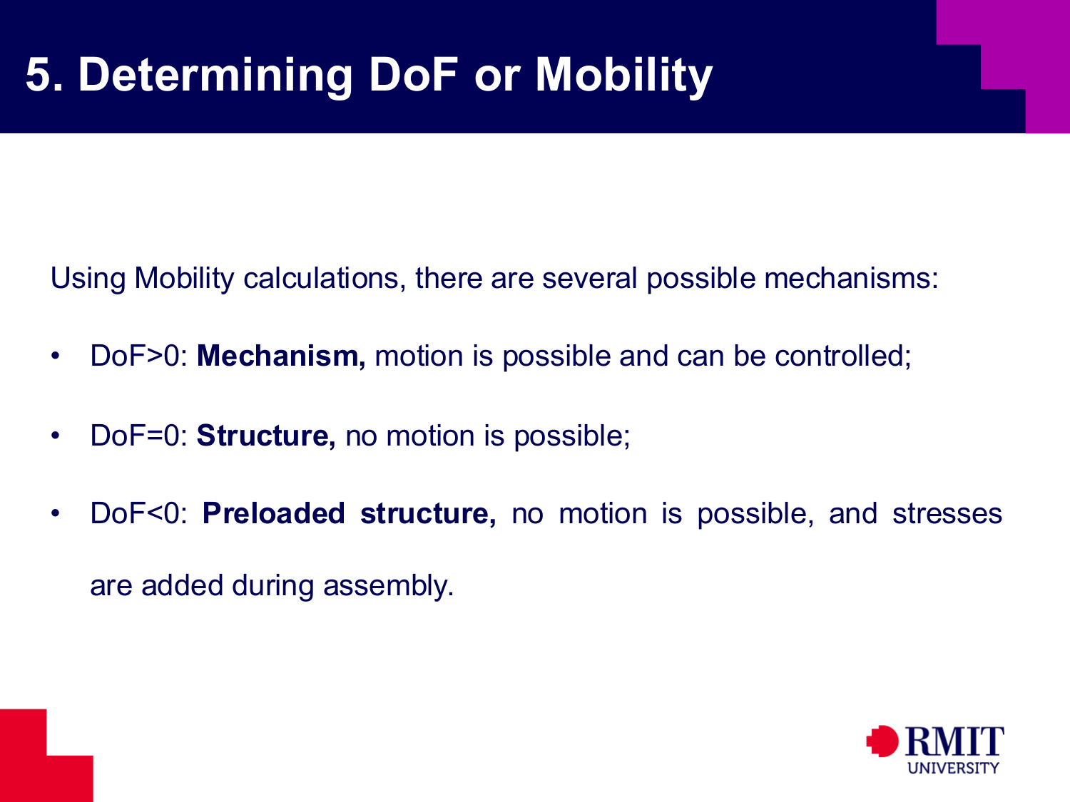
The value of $M$ describes the assembly. If $M>0$, at least one independent motion is possible and the assembly is a mechanism. If $M=0$, no motion is possible and the assembly is a structure. If $M<0$, there are too many constraints. Closing or assembling it then creates internal stress.

An exactly constrained system has only the constraints needed for the intended behaviour. Extra constraints make the system sensitive to manufacturing errors because its parts may need to deform during assembly.

A correct mobility calculation begins with correct counting. Identify all links, full joints and half joints before interpreting $M$. Even a small counting error can make a mechanism appear to be a structure in the calculation.

An external body may need to be counted as another link when it affects the motion. A held object, contact surface or slider block becomes part of the kinematic model if it adds a constraint.

Mobility can therefore change when contact begins or ends. A device may have one degree of freedom before contact and become a structure after contact if enough new constraints are added.

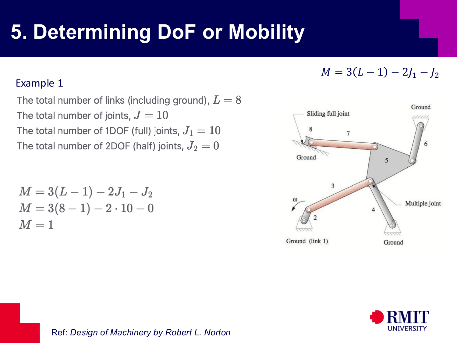
For $L=8$, $J_1=10$, and $J_2=0$, \(M = 3(8-1) - 2(10) - 0 = 1.\) This mechanism has one independent input. Many planar machines use this design because one known input determines the position of the whole assembly.

The method still works with multiple joints, but they must be counted correctly. A pin shared by three links adds more constraints than a pin joining two links.

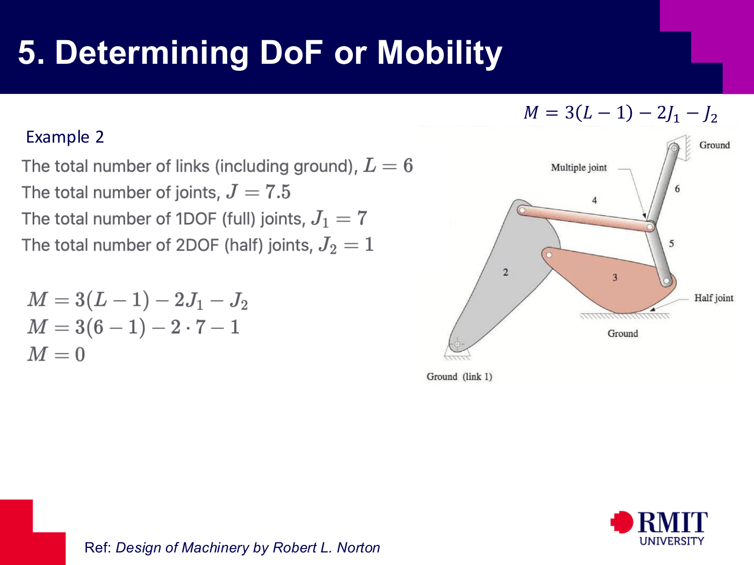
A half joint removes less motion than a full joint and must be counted separately. With $L=6$, $J_1=7$, and $J_2=1$, \(M = 3(6-1) - 2(7) - 1 = 0,\) so the assembly is classified as a structure rather than as a moving mechanism.

This example shows why full and half joints are counted differently. Multiple joints can make the count look unusual. Fractional values may appear in intermediate counts when equivalent first-order joints represent a shared connection.

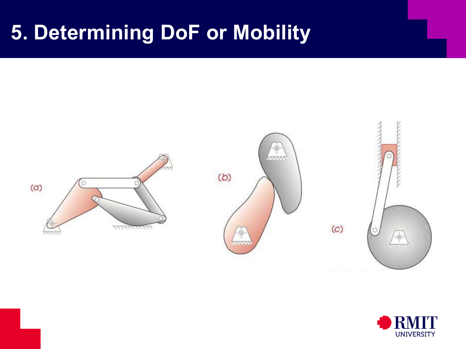
To calculate mobility, identify the ground link, full joints, half joints and multiple joints from the chain geometry. Mechanisms may look different, but the counting method remains the same.

First draw or imagine the kinematic diagram. Then count the links, classify the joints and finally use the mobility equation. Counting directly from a complex product image is more likely to cause errors.

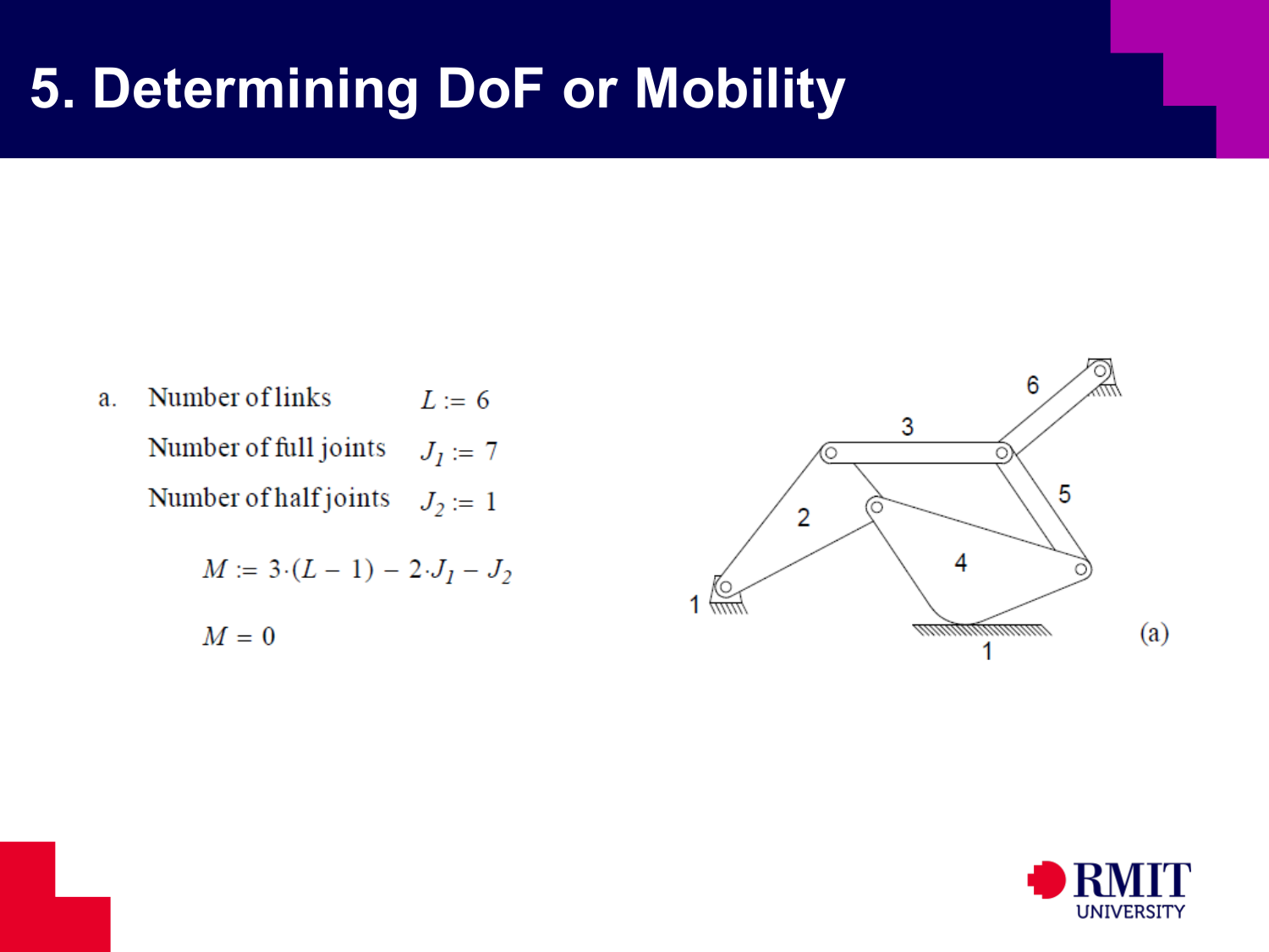
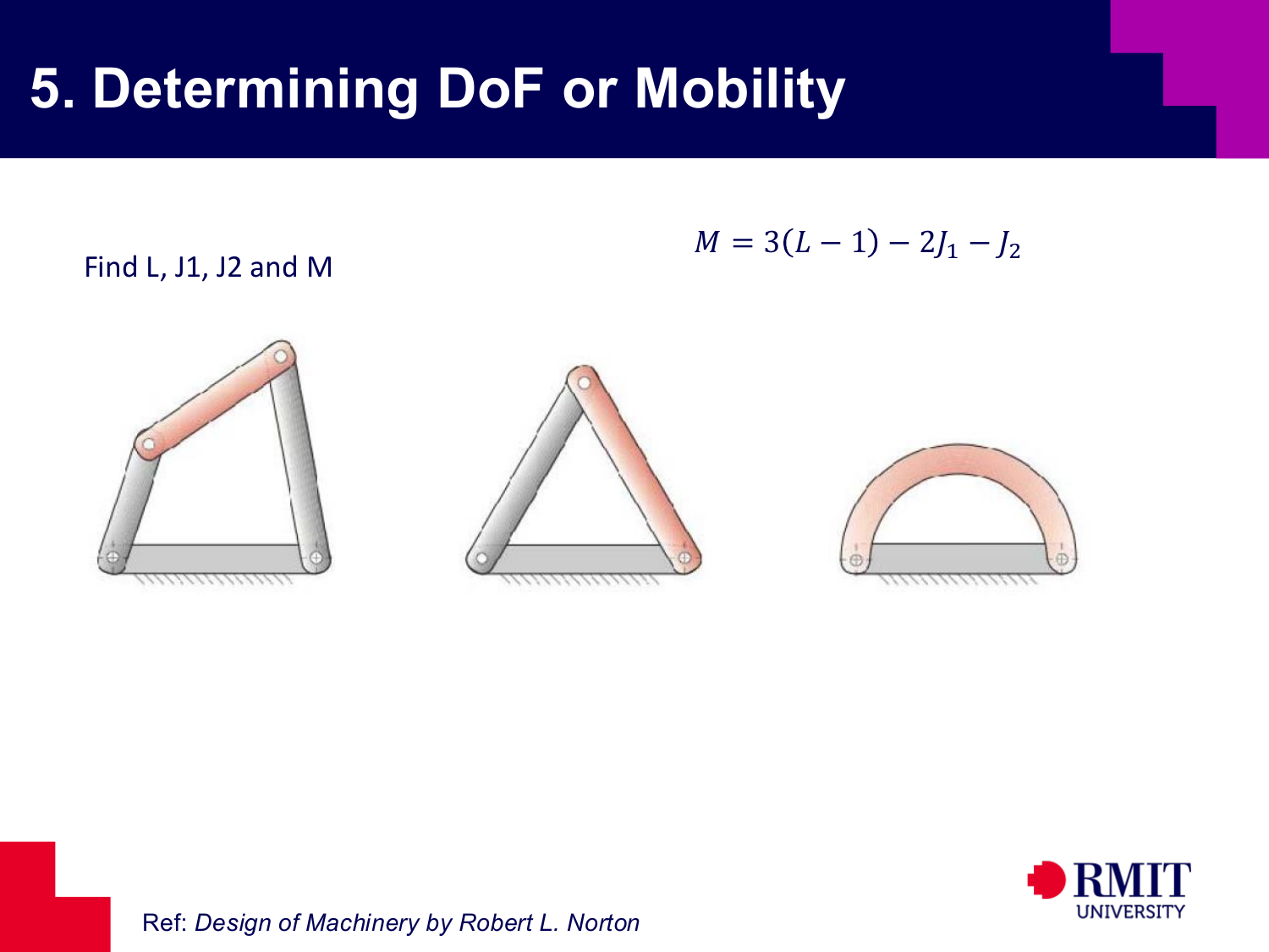
For example (a), the counts $L=6$, $J_1=7$, and $J_2=1$ lead to \(M = 3(6-1) - 2(7) - 1 = 0,\) so the assembly is a structure. A complex appearance does not mean that an assembly can move. Mobility depends on the balance between possible motion and constraints.

The example also shows that a structure with zero degrees of freedom can contain a multiple joint. Count the constraints instead of judging the figure by its appearance.

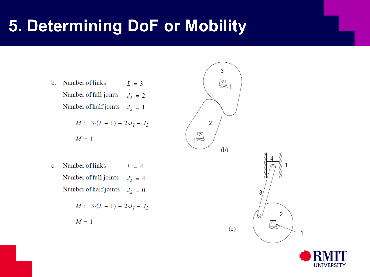
Examples (b) and (c) both have one degree of freedom. For (b), $L=3$, $J_1=2$ and $J_2=1$ give $M=1$. For (c), $L=4$, $J_1=4$ and $J_2=0$ also give $M=1$. Different layouts can therefore have the same mobility even when they do not look similar.

Equivalent mobility does not imply identical motion paths or identical force transmission. It means only that the number of independent inputs is the same.

Planar mechanism analysis connects several ideas. Degree of freedom gives the amount of independent motion. Motion types describe how bodies move. Links and joints create constraints. Kinematic diagrams simplify the system, and mobility equations give a numerical result.

Understanding mobility requires clear definitions and repeated calculations. Use the terms for links, joints and motion consistently so that the final degree-of-freedom count has a clear physical meaning.

In practice, the most common sources of error are omitting the ground link, misclassifying a half joint as a full joint, and overlooking the special treatment required by a multiple joint or by a constrained external body.

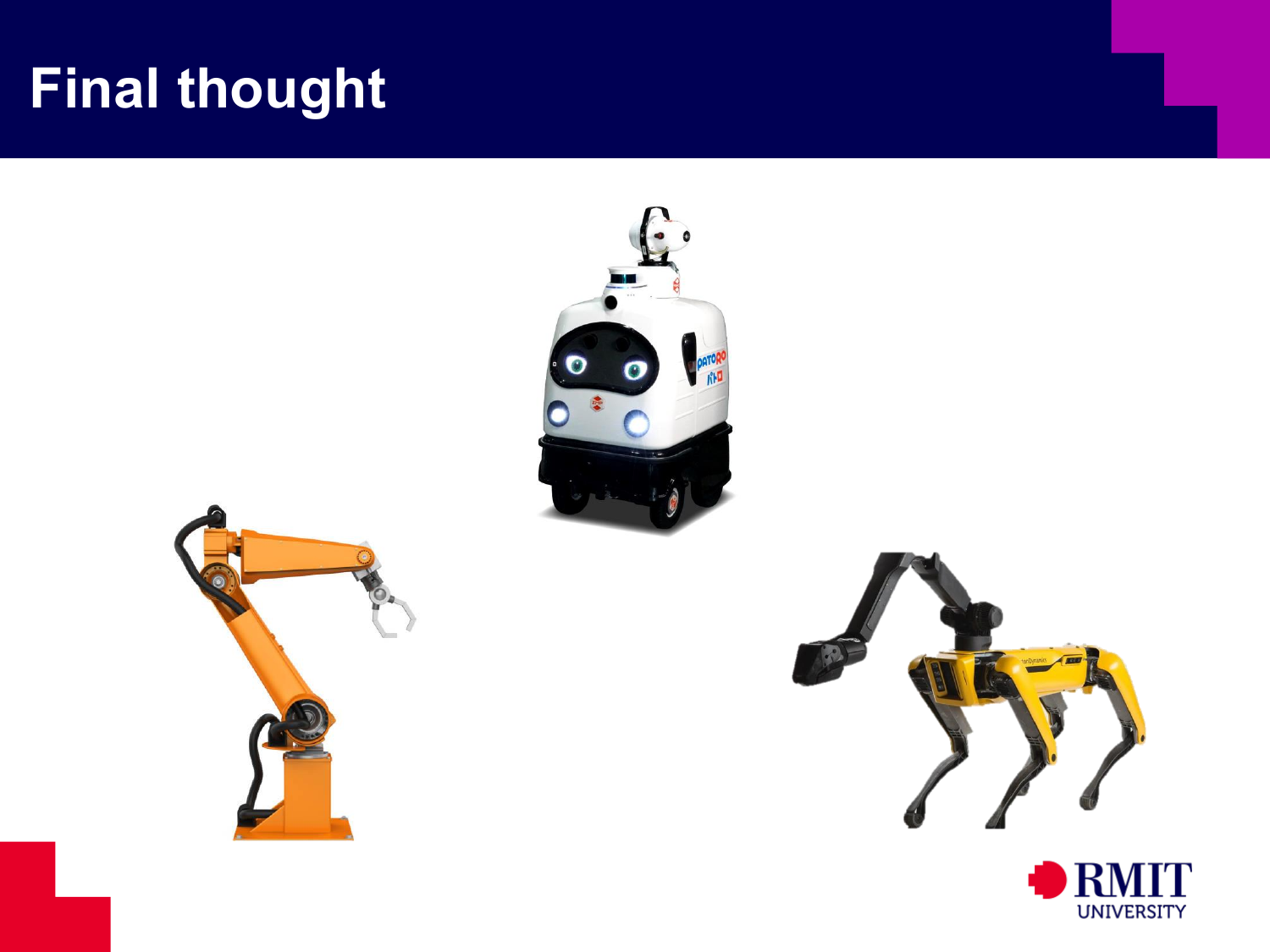
Modern robots use the same ideas. In an industrial robot, mobile robot or legged robot, the arrangement of rigid links, joints, constraints and actuators determines the motion.

[For Illustration Only]

[For Illustration Only]

[For Illustration Only]

[For Illustration Only]

The second part covers number synthesis, mechanism paradoxes and linkage transformation. It examines how a mechanism structure can be created, changed or incorrectly understood.

Number synthesis determines the number and order of links and joints needed for a chosen degree of freedom. Binary, ternary, quaternary and higher-order links must be counted consistently by their number of nodes.

The purpose is to find possible connection patterns before choosing the detailed dimensions.

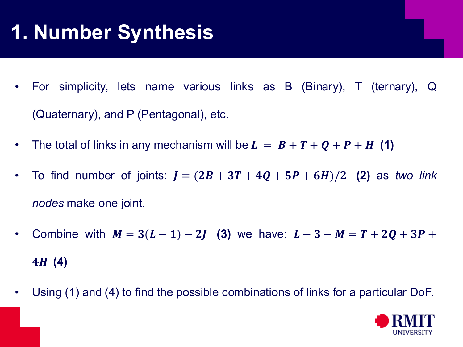
Mechanism synthesis can be organised through a counting framework: \(L = B + T + Q + P + H,\) \(J = \frac{2B + 3T + 4Q + 5P + 6H}{2},\) and, for planar full-joint chains, \(M = 3(L - 1) - 2J.\) Combining these relations gives \(L - 3 - M = T + 2Q + 3P + 4H,\) These equations identify possible combinations of link orders for a chosen degree of freedom. They also show how the number of joints depends on the link orders.

For planar chains with only full joints, mobility and link count have opposite parity. Odd mobility requires an even number of links, while even mobility requires an odd number. This rule reduces the number of possible linkage structures.

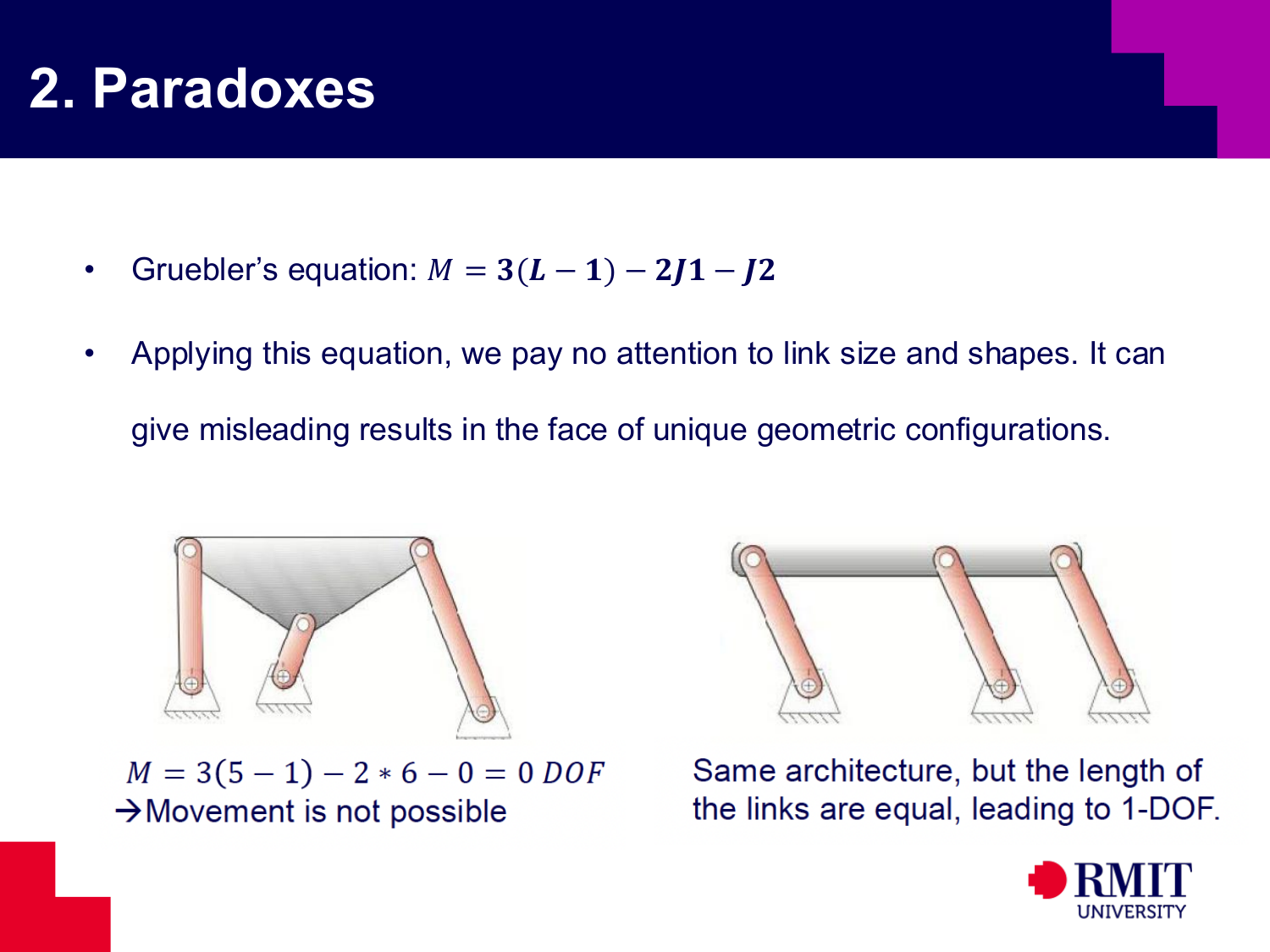
Gruebler’s equation counts the structure but does not fully test the geometry. It ignores exact dimensions and special arrangements, so its predicted mobility may be incorrect. A mechanism paradox occurs when the geometry adds hidden constraints or allows unexpected motion that the counting equation cannot detect.

Transformation rules help compare related planar chains. Replacing a revolute joint in a loop with a prismatic joint can leave mobility unchanged if enough revolute joints remain. Replacing a full joint with a half joint increases mobility by $1$. Removing a link decreases mobility by $1$.

These rules show that appearance does not determine kinematic behaviour. Two mechanisms can look different but have the same number of constraints.

Combined changes can also keep mobility unchanged. Replacing a full joint with a half joint and then removing a link can keep the same degree of freedom. Shrinking a higher-order link by joining its nodes can create multiple joints without changing mobility. However, completely shrinking the link is the same as removing it and reduces mobility.

Higher-order links must therefore be identified correctly. Their role depends on the number and arrangement of nodes, not only on their shape.

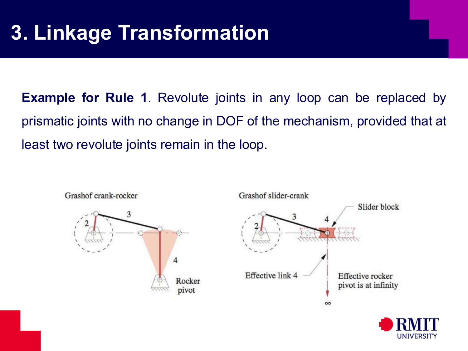
A Grashof crank-rocker and a Grashof slider-crank can have the same mobility. One uses only revolute joints, while the other also uses a prismatic joint. Degree of freedom depends on the constraint structure, not on the physical appearance.

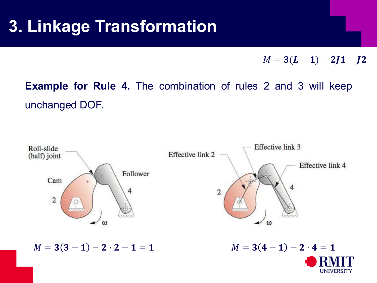
Applying the relevant transformation sequence changes the description of links and joints, but the mechanism remains equivalent in mobility: \(M = 1,\) so the same single independent motion is retained after transformation.

[For Illustration Only]

[For Illustration Only]

[For Illustration Only]

Knowledge Check