Acceleration Analysis (Vector Loop Method)
Four-Bar Crank-Slider Vector Loop Equations
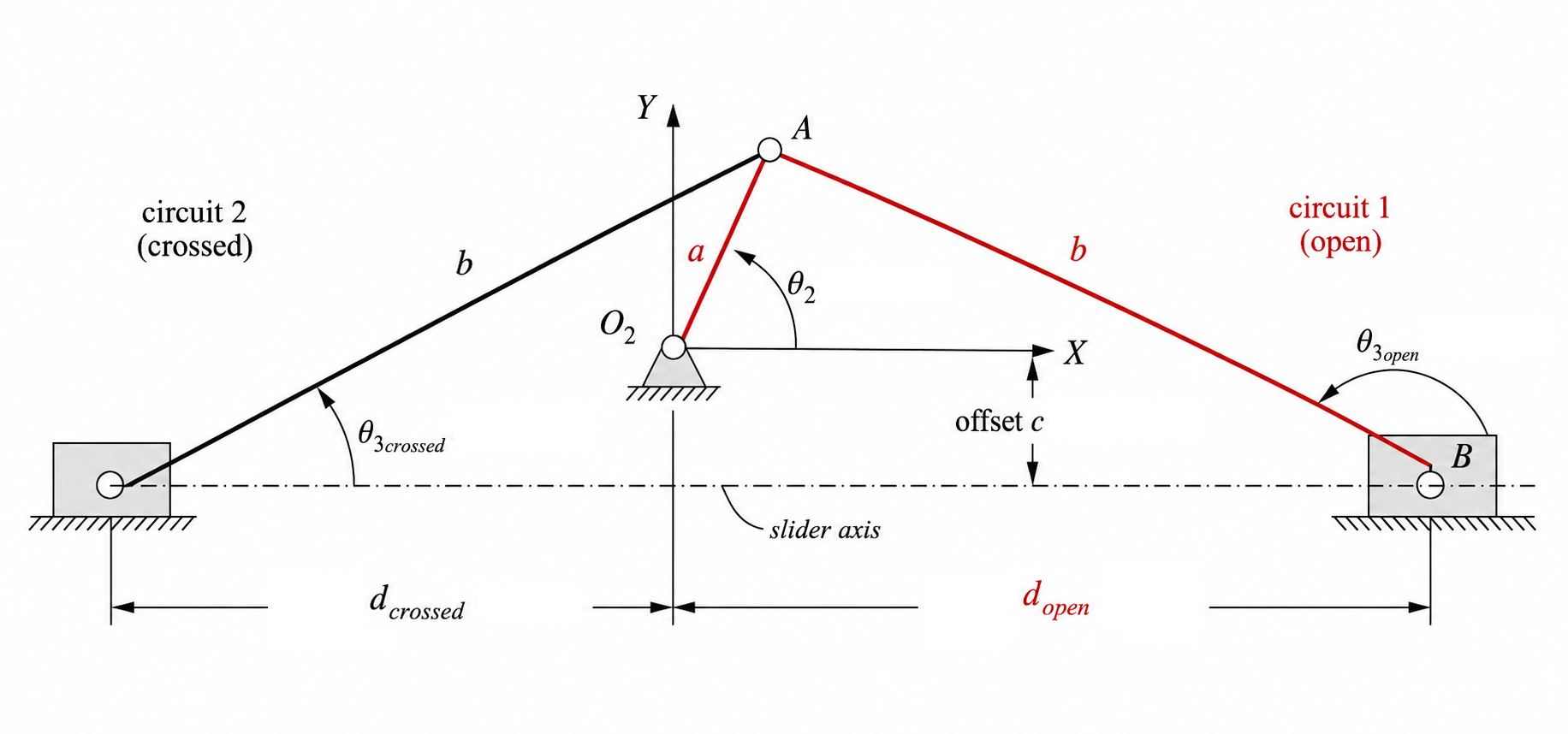
The derivation of the vector loop equation for a four-bar crank-slider mechanism follows the same closure logic as the four-bar linkage, except that one end point is constrained to move on a straight guide. In the notation used here, the crank has length $a$, the coupler has length $b$, the slider position is $d$, and $c$ is the signed vertical offset of the slider axis relative to $O_2$. Thus $c<0$ when the slider axis is below $O_2$ and $c>0$ when it is above $O_2$.
Vector Loop Equation
Traversing the mechanism from the grounded crank pivot to the slider pin gives the closure statement
\[\mathbf{R}_A+\mathbf{R}_{BA}-\mathbf{R}_{BO_2}=0.\]Using complex notation for the rotating links and Cartesian form for the slider position gives
\[a e^{j\theta_2}-b e^{j\theta_3}-(d+jc)=0\]where the slider position vector is $\mathbf{R}_{BO_2}=d+jc$. The offset $c$ is constant for a fixed guide.
Using Euler’s relation, $e^{j\theta}=\cos\theta+j\sin\theta$, this becomes
\[a(\cos\theta_2+j\sin\theta_2)-b(\cos\theta_3+j\sin\theta_3)-(d+jc)=0.\]Solving for Accelerations
Determining accelerations from the crank-slider vector loop follows the same structure as the position and velocity analyses. Once the current geometry and velocities are known, differentiating once more gives the instantaneous angular acceleration of the coupler and the slider acceleration.
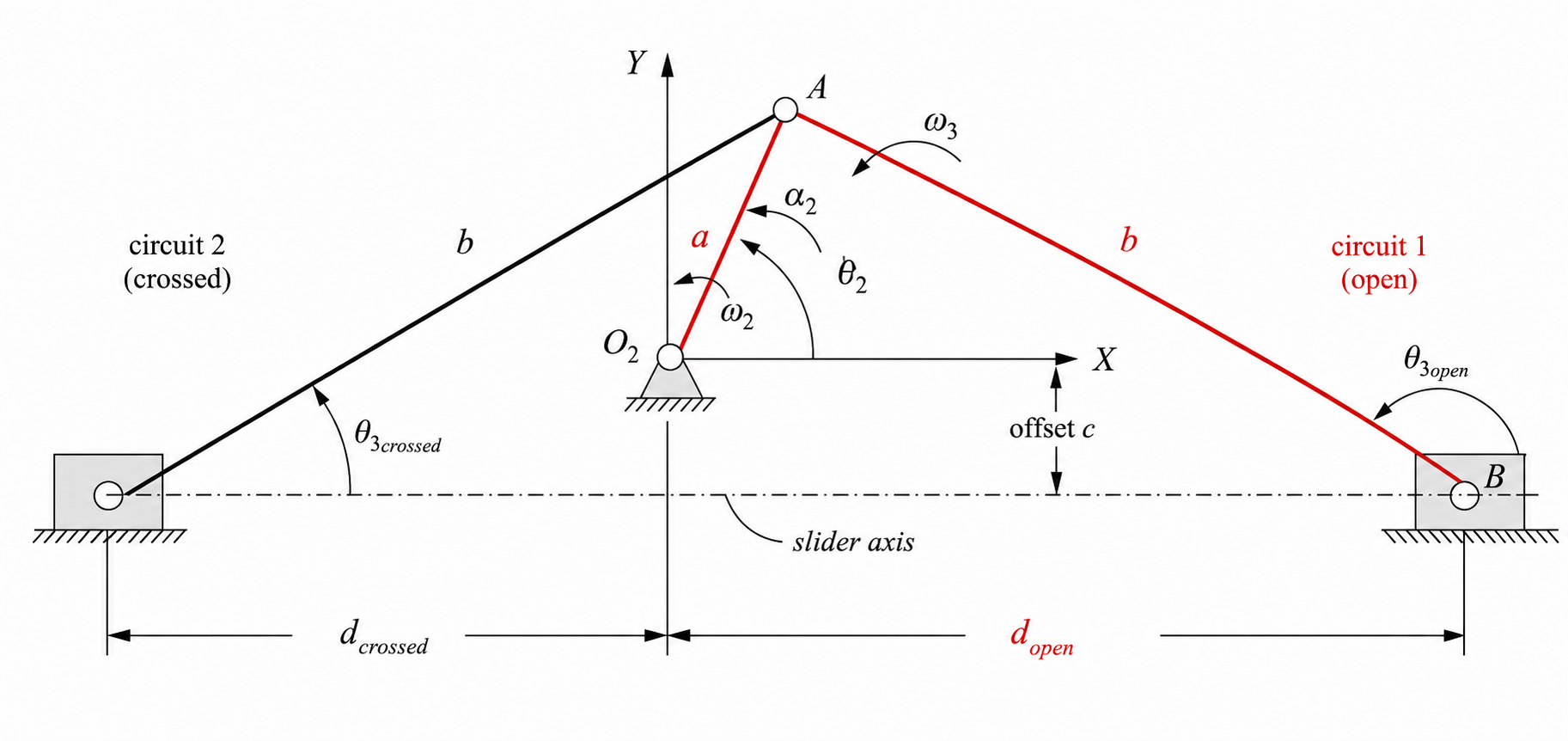
Previously, in Velocity Analysis we differentiated the position loop to obtain
\[j a \omega_2 e^{j\theta_2}-j b \omega_3 e^{j\theta_3}-\dot d=0.\]Differentiating once more with respect to time gives
\[a(j\alpha_2-\omega_2^2)e^{j\theta_2} -b(j\alpha_3-\omega_3^2)e^{j\theta_3} -\ddot d=0.\]This equation contains both tangential terms proportional to $\alpha$ and normal terms proportional to $\omega^2$. The slider term remains purely real because its motion is constrained to the guide axis.
Using Euler’s relation gives
\[\begin{aligned} &a(j\alpha_2-\omega_2^2)(\cos\theta_2+j\sin\theta_2) \\ &\quad-b(j\alpha_3-\omega_3^2)(\cos\theta_3+j\sin\theta_3)-\ddot d=0. \end{aligned}\]Using
\[(j\alpha-\omega^2)(\cos\theta+j\sin\theta) = (-\alpha\sin\theta-\omega^2\cos\theta) + j(\alpha\cos\theta-\omega^2\sin\theta),\]the acceleration loop simplifies to
\[\begin{aligned} &a(-\alpha_2\sin\theta_2-\omega_2^2\cos\theta_2+j(\alpha_2\cos\theta_2-\omega_2^2\sin\theta_2)) \\ &\quad-b(-\alpha_3\sin\theta_3-\omega_3^2\cos\theta_3+j(\alpha_3\cos\theta_3-\omega_3^2\sin\theta_3))-\ddot d=0. \end{aligned}\]Separating into real and imaginary components gives, first, the real part:
\[-a\alpha_2\sin\theta_2-a\omega_2^2\cos\theta_2+b\alpha_3\sin\theta_3+b\omega_3^2\cos\theta_3-\ddot d=0\]and second, the imaginary part:
\[a\alpha_2\cos\theta_2-a\omega_2^2\sin\theta_2-b\alpha_3\cos\theta_3+b\omega_3^2\sin\theta_3=0.\]The imaginary equation can be solved first for the coupler angular acceleration:
\[b\alpha_3\cos\theta_3 = a\alpha_2\cos\theta_2-a\omega_2^2\sin\theta_2+b\omega_3^2\sin\theta_3\] \[\alpha_3 = \frac{a\alpha_2\cos\theta_2-a\omega_2^2\sin\theta_2+b\omega_3^2\sin\theta_3}{b\cos\theta_3}.\]Substituting $\alpha_3$ into the real equation gives the slider acceleration:
\[\ddot d=-a\alpha_2\sin\theta_2-a\omega_2^2\cos\theta_2+b\alpha_3\sin\theta_3+b\omega_3^2\cos\theta_3.\]Point Accelerations
The point accelerations that remain useful for later dynamic-force analysis are
\[\mathbf{A}_A = a\alpha_2(-\sin\theta_2+j\cos\theta_2) -a\omega_2^2(\cos\theta_2+j\sin\theta_2),\] \[\mathbf{A}_{BA} = -b\alpha_3(-\sin\theta_3+j\cos\theta_3) +b\omega_3^2(\cos\theta_3+j\sin\theta_3),\] \[\mathbf{A}_B=\ddot d\,\hat{\mathbf{i}}.\]The minus sign in $\mathbf{A}_{BA}$ comes from the same sign convention used in the position loop, where $\mathbf{R}_{BA}=-b e^{j\theta_3}$. The acceleration of point $B$ is purely horizontal in this coordinate system, which again reflects the guide constraint. This is the key simplification that distinguishes the crank-slider from the conventional four-bar in acceleration analysis.