Lecture 2: Kinematic Analysis of Mechanism

[For Illustration Only]

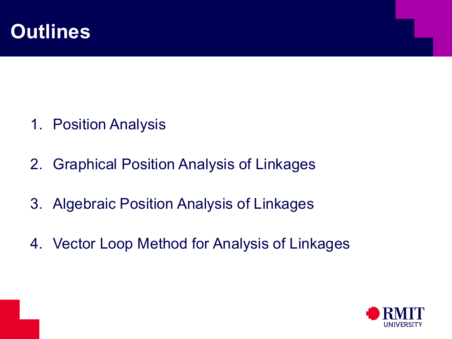
Part 1 covers four connected topics: position analysis, graphical position analysis, algebraic position analysis and the vector-loop method. Each method expresses the same geometric closure conditions in a different way.

The aim is to develop a method that can be used for different mechanisms. Graphical construction shows the possible positions. Algebraic methods solve for unknown point locations. The vector-loop method gives a compact equation that can later be differentiated to find velocity and acceleration.

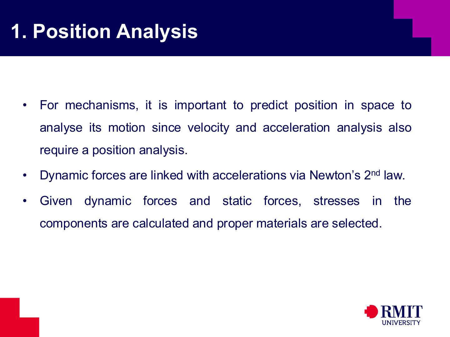
Position analysis is the starting point for most kinematic and dynamic calculations. Differentiating position with respect to time gives velocity. Differentiating velocity gives acceleration. Dynamic forces depend on acceleration through Newton’s second law, so force and stress calculations first need a correct position model.

For a mechanism in continuous operation, its position must be found at more than one input angle. The equations must describe the mechanism throughout its motion cycle, not only at one drawn position.

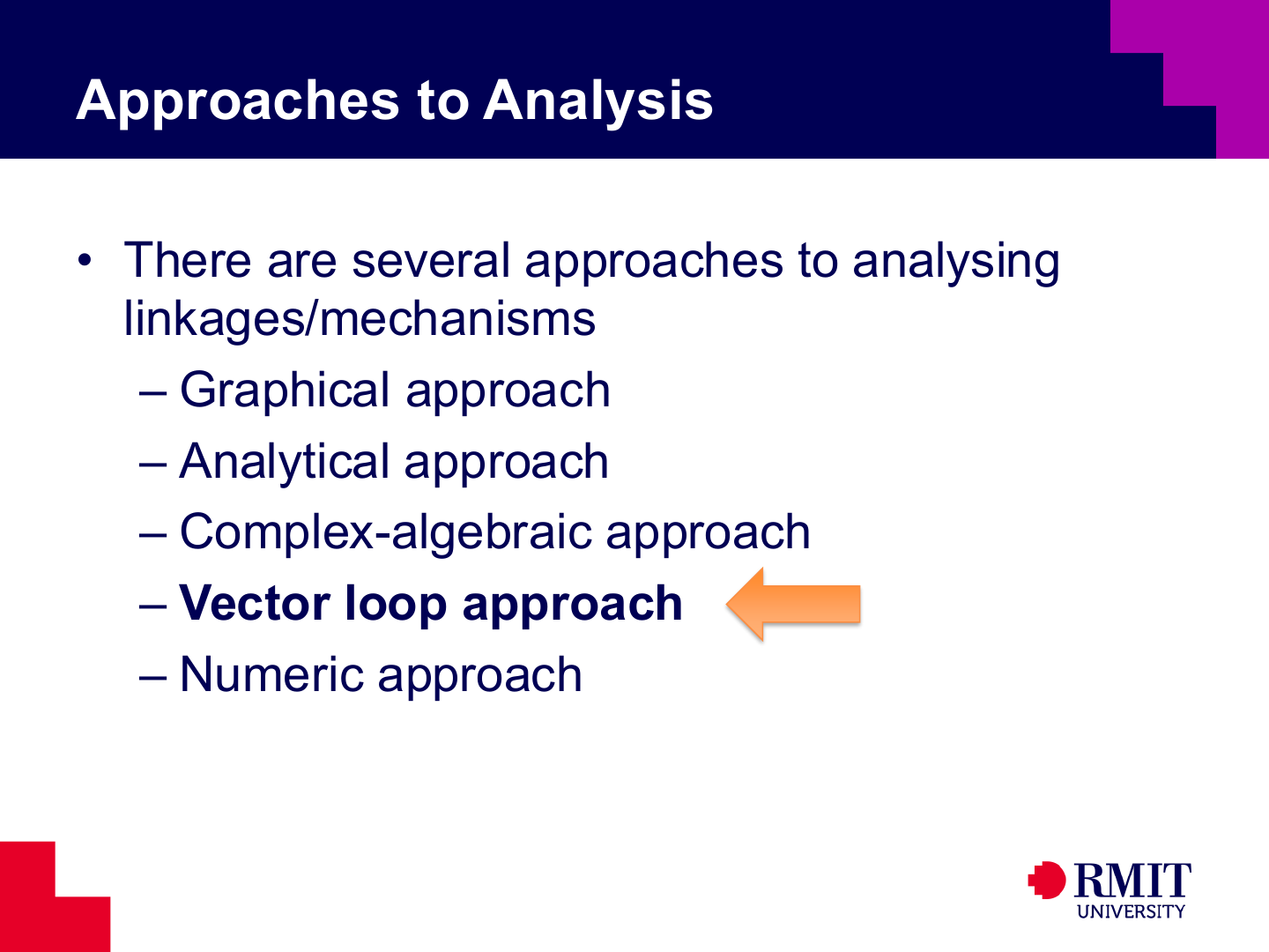
Linkages can be analysed using graphical, algebraic, complex-number, vector-loop or numerical methods. Each method represents the same constraints in a different way.

Graphical methods help show the geometry and provide a quick solution. Algebraic and vector-loop methods provide a clear calculation process. Numerical methods are useful when a mechanism is too complex to solve by hand with a single formula.

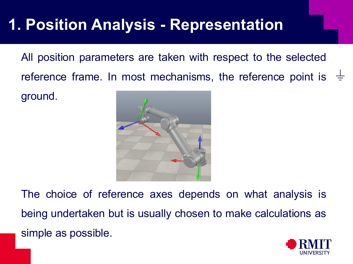
All position variables must be defined relative to a chosen reference frame, and the ground link is the usual reference in mechanism analysis.

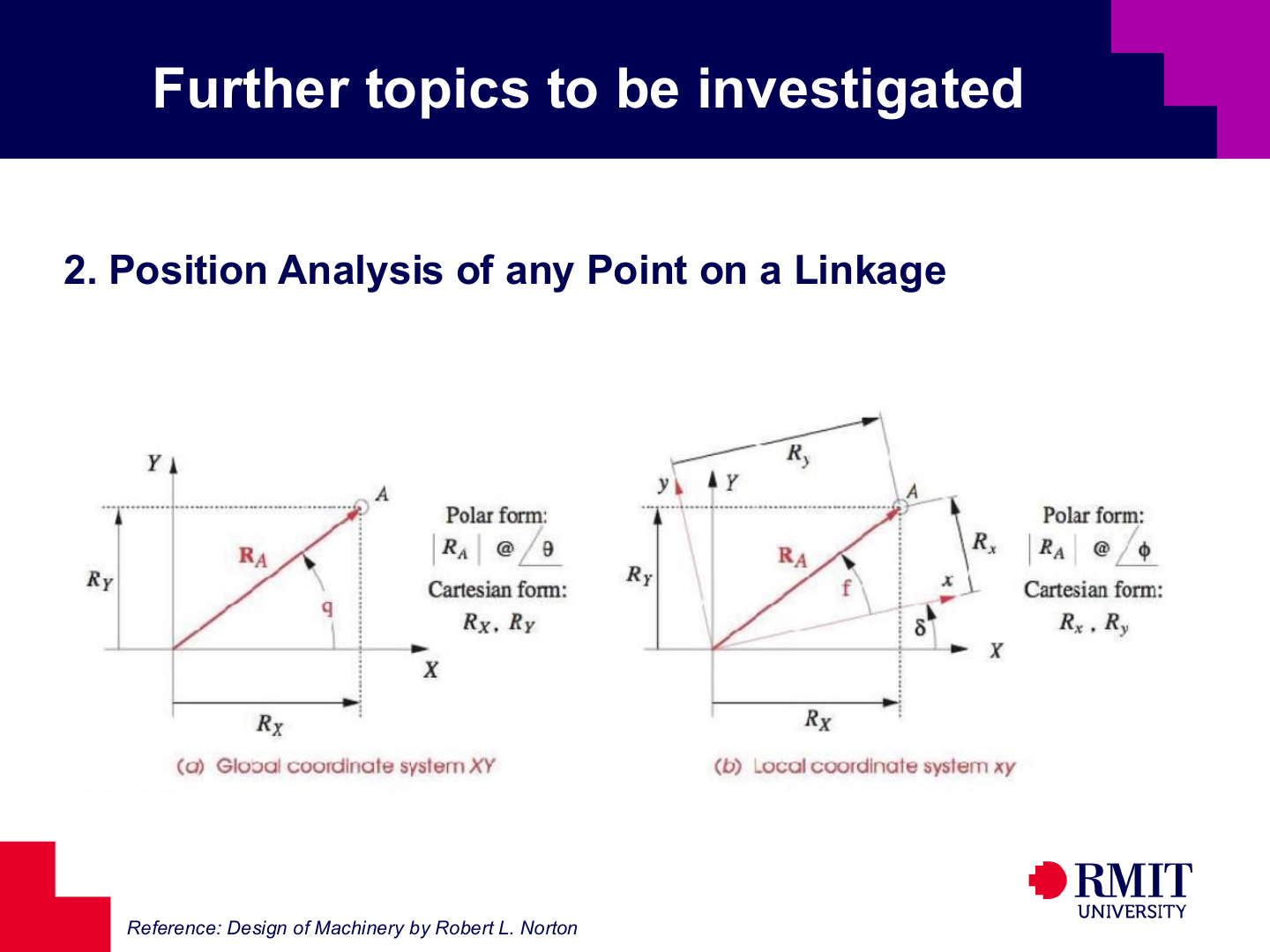
A two-dimensional position vector can use polar form, with a magnitude and angle, or Cartesian form, with $x$ and $y$ components. Either form describes the same vector.

The choice of coordinates does not change the physics. However, aligning an axis with a known motion, fixed pivot or slider direction can make the equations much simpler.

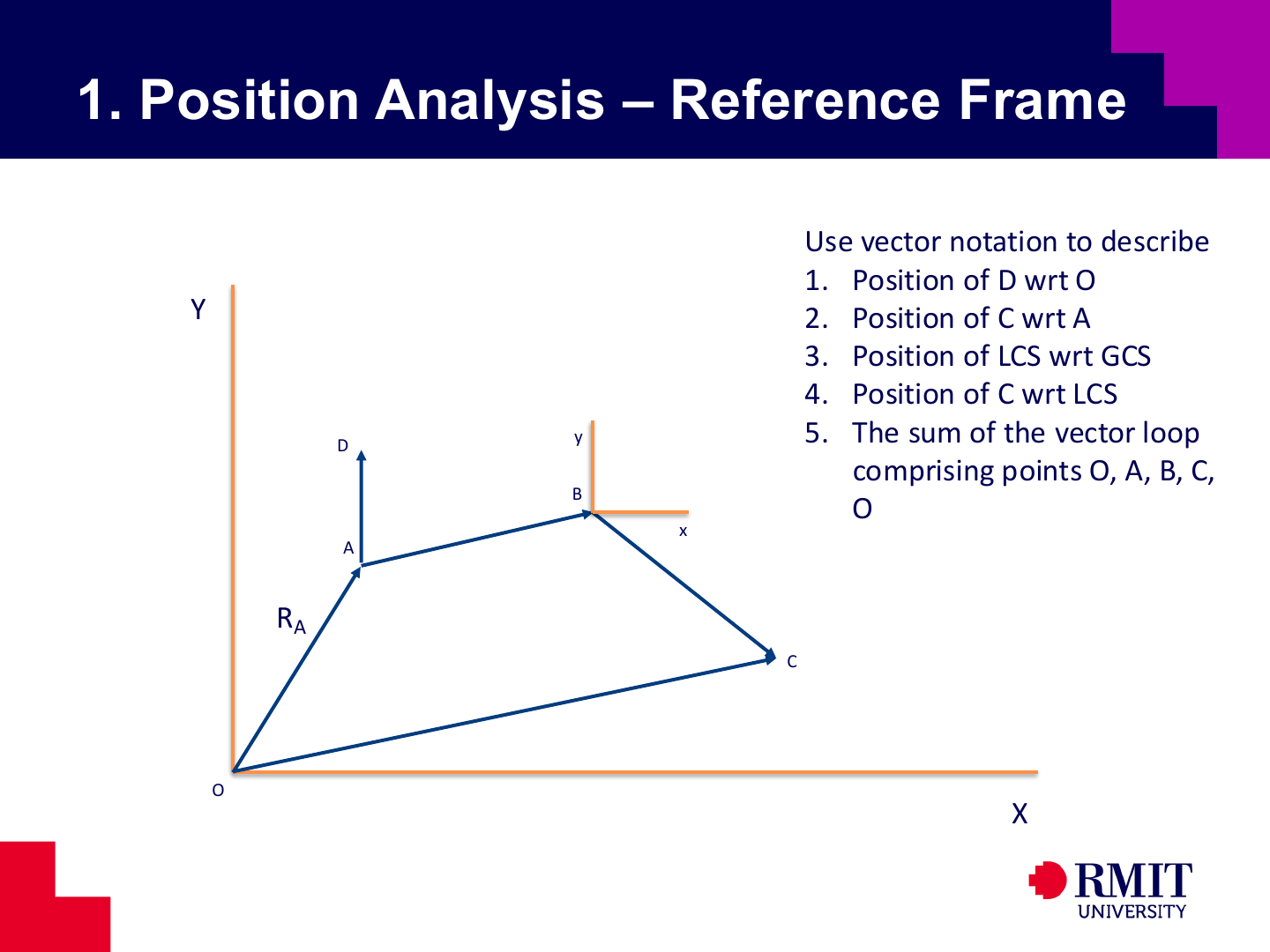
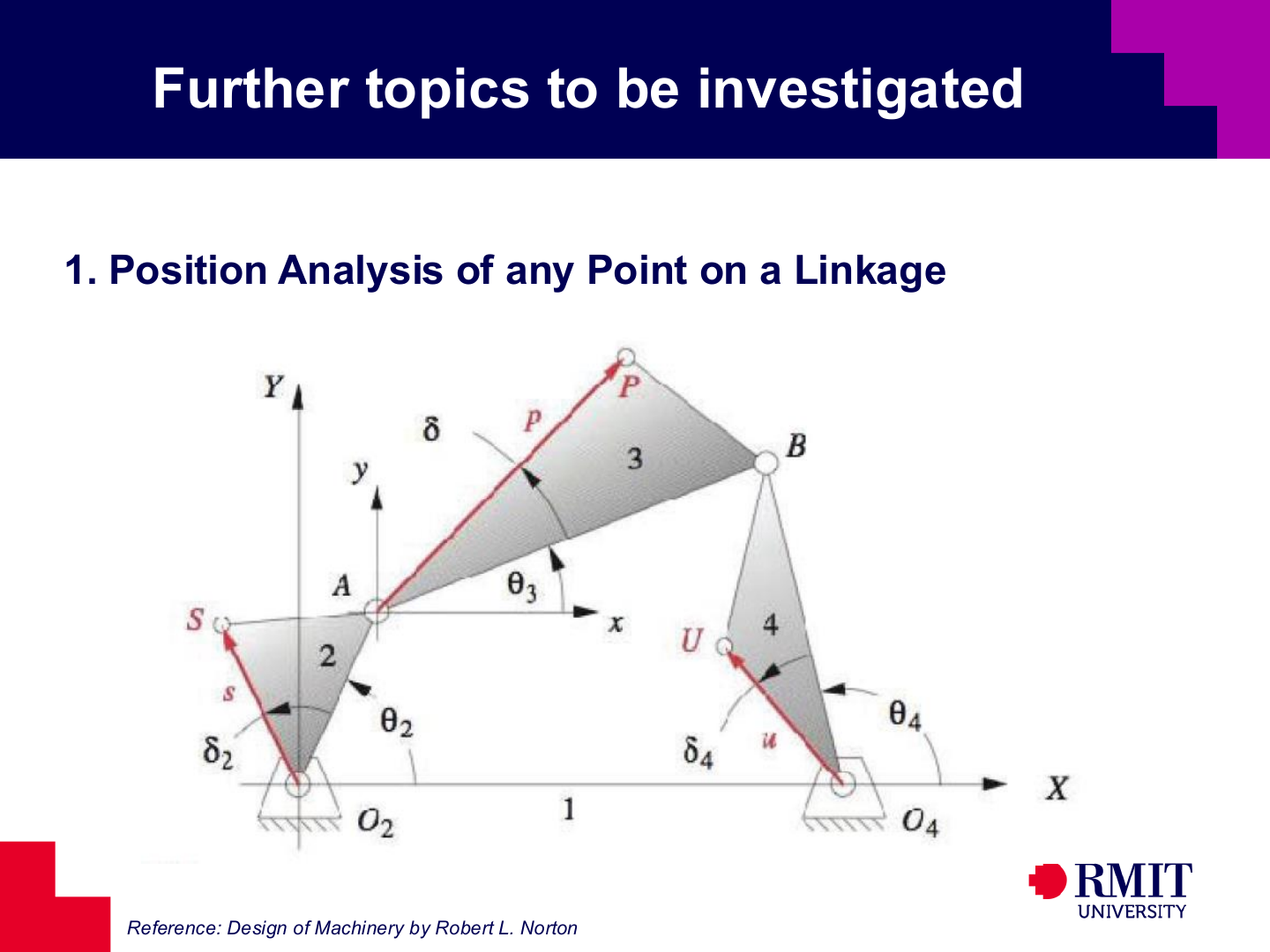
Vectors between named points describe positions in a mechanism. They can show the position of $D$ relative to $O$, the position of $C$ relative to $A$, and the relationship between local and global coordinates.

Tracing a closed path around a linkage must return to the starting point, so the vector sum is zero. This loop-closure rule changes the linkage geometry into equations that must be true at every possible position.

Using the notation shown in the figure, the requested vector descriptions are:

1. Position of $D$ with respect to $O$: $\mathbf{R}_{DO}$
2. Position of $C$ with respect to $A$: $\mathbf{R}_{CA}$
3. Position of the local-origin point with respect to the global origin: $\mathbf{R}_{O_{\ell}O}$
4. Position of $C$ with respect to the local origin: $\mathbf{R}_{CO_{\ell}}$
5. For the closed loop passing through the points $O$, $A$, $B$, $C$, and back to $O$, the loop-closure condition is: $\mathbf{R}_{AO}+\mathbf{R}_{BA}+\mathbf{R}_{CB}+\mathbf{R}_{OC}=\mathbf{0}$.

An equivalent form is $\mathbf{R}_{OA}+\mathbf{R}_{AB}+\mathbf{R}_{BC}+\mathbf{R}_{CO}=\mathbf{0}$, provided that the subscripts follow the chosen direction around the loop.

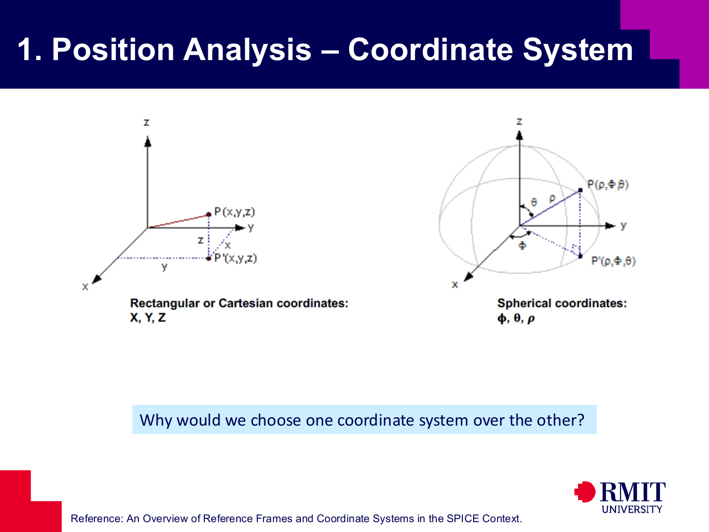
The best coordinate system depends on the calculation. A global coordinate system describes the whole mechanism. A local coordinate system is often easier for a point fixed to a moving link.

Choose the reference frame that makes the constraints easiest to express. Aligning an axis with a slider, fixed pivot or known line of motion often shortens the calculation and reduces sign errors.

If local coordinates $(R_x,R_y)$ are known and the local axes are rotated by an angle $\delta$ relative to the global axes, then a pure rotation of components gives

\[\begin{aligned} R_X &= R_x \cos \delta - R_y \sin \delta, \\ R_Y &= R_x \sin \delta + R_y \cos \delta \end{aligned}\]

This form is valid when the local and global origins coincide. More generally, if the local origin has global coordinates $(X_{O_{\ell}},Y_{O_{\ell}})$, then the full coordinate transformation is

\[\begin{aligned} R_X &= X_{O_{\ell}} + R_x \cos \delta - R_y \sin \delta, \\ R_Y &= Y_{O_{\ell}} + R_x \sin \delta + R_y \cos \delta \end{aligned}\]

This transformation is used repeatedly when points are fixed on moving links.

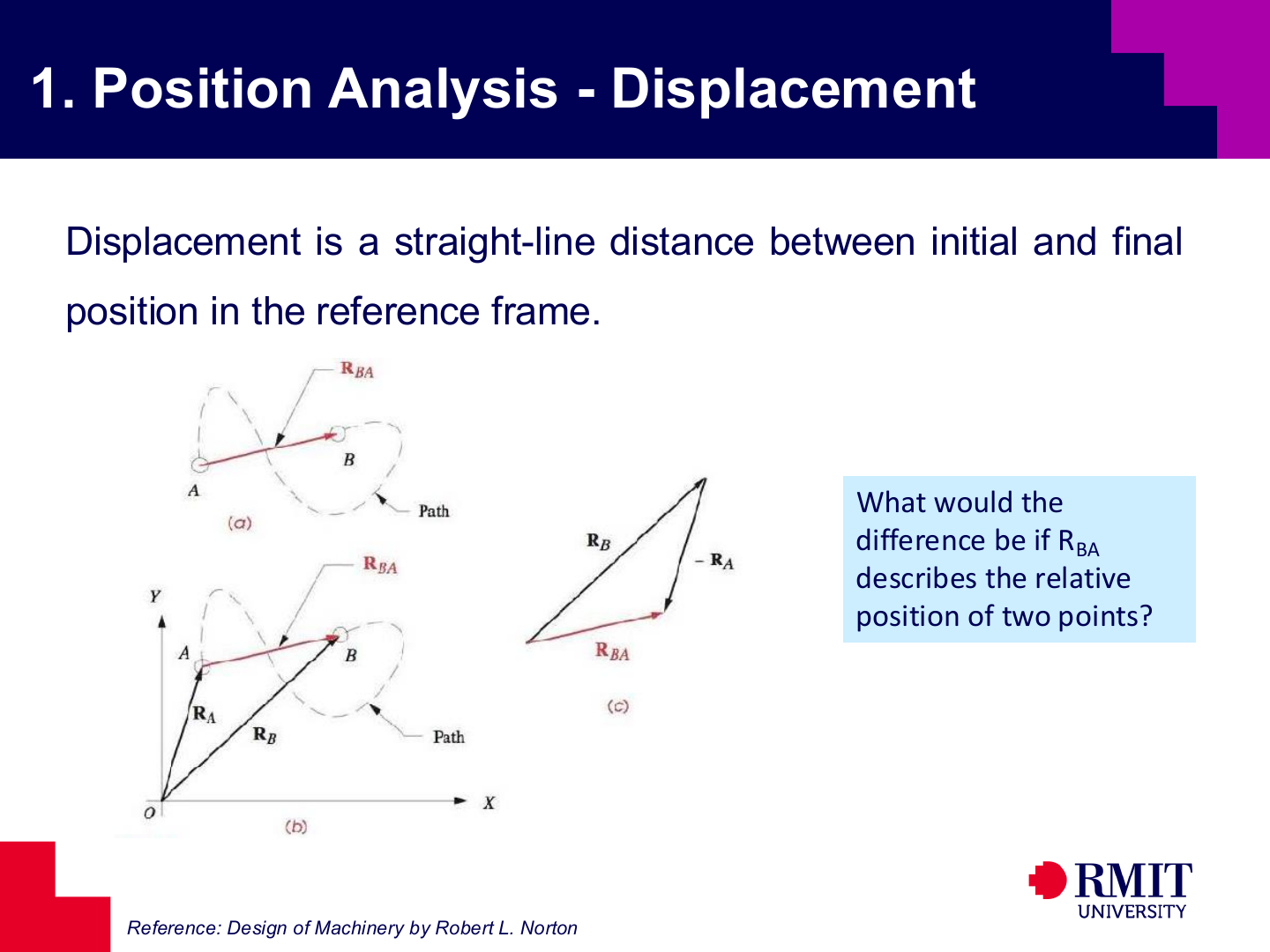
Displacement is the change in a point’s position from its initial position to its final position, measured in the selected reference frame.

Relative position describes one point from another point at the same instant. Both use the same vector subtraction: $\mathbf{R}_{BA} = \mathbf{R}_{B} - \mathbf{R}_{A}.$

The meaning depends on whether $A$ and $B$ are two positions of one body at different times or the positions of two bodies at the same time.

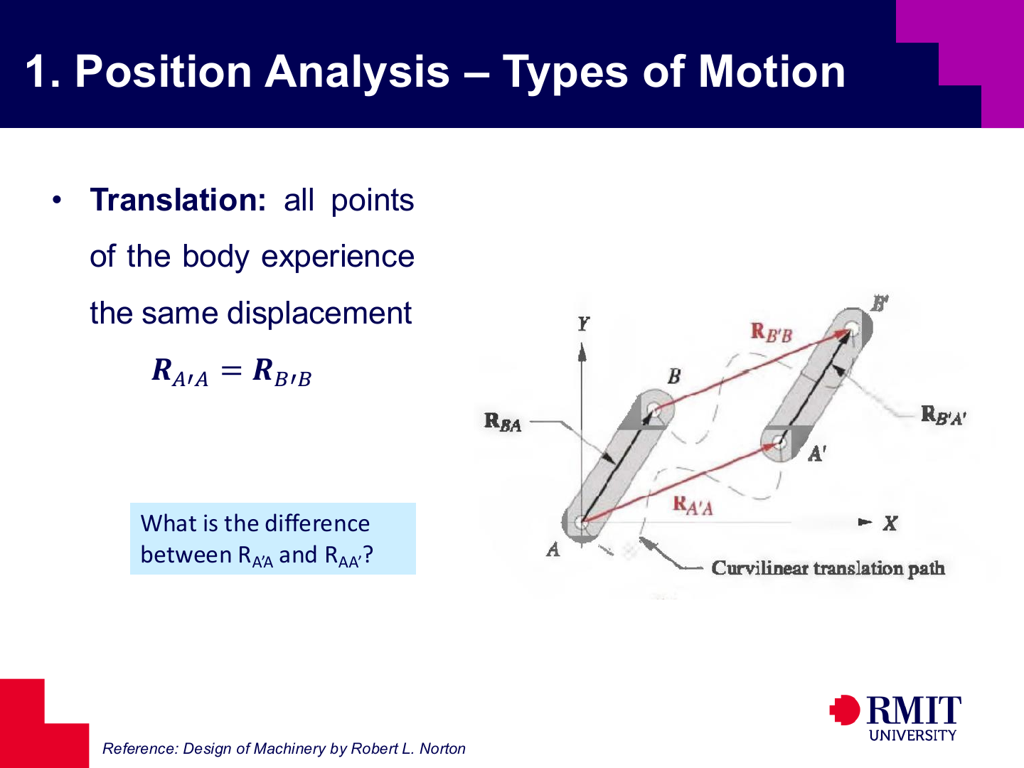
For pure translation, every point on the rigid body has the same displacement. For matching points on the body, $\mathbf{R}_{A^{\prime}A}=\mathbf{R}_{B^{\prime}B}.$

The body does not rotate during pure translation. Its orientation remains unchanged, and all points have the same displacement.

Translation does not need to follow a straight line. Curvilinear translation follows a curved path, while rectilinear translation follows a straight path.

The notation order matters because reversing the subscripts reverses the vector direction and therefore changes the sign. Thus $\mathbf{R}_{AA^{\prime}}=-\mathbf{R}_{A^{\prime}A}.$

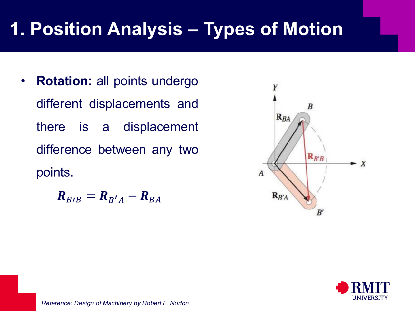
During pure rotation, points on the same body usually have different displacements. One point or axis remains fixed, while all other points move in circular paths around the centre of rotation.

One displacement vector therefore cannot describe every point on the body. For the same rotation angle, a point near the centre follows a shorter arc than a point farther away. If the body rotates through $\theta$, a point at radius $r$ moves through the arc length $s=r\theta.$

The displacement therefore depends on the position of the point within the body, not just on the fact that the body has rotated.

Displacement equations for rotation must use the relative position of each point. In translation, all points have the same displacement vector. In rotation, each point’s motion depends on its distance and direction from the centre of rotation or another reference point.

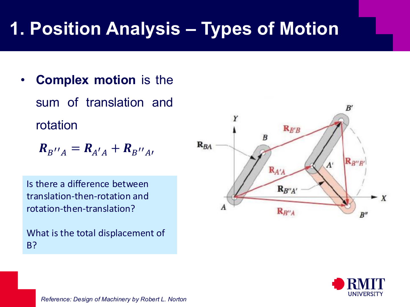
Complex planar motion combines translation and rotation. The total motion of a point combines body translation with rotation about a moving point or frame. Both motions must use the same reference frame before they are added.

Coupler links in planar mechanisms usually have complex motion. Chasles’ theorem states that this motion can be represented by translating one point on the body and rotating the body about that point.

The order of these operations is important. Translation followed by rotation usually gives a different final position from rotation followed by translation. The sequence of motions must therefore be clearly defined.

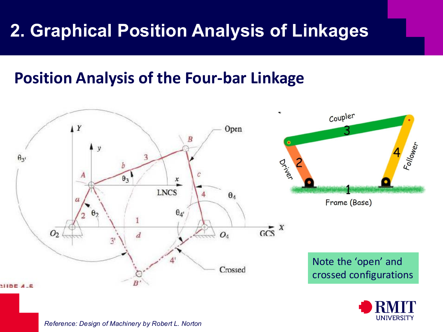
Graphical position analysis uses a geometric drawing to find an unknown linkage position. For a four-bar mechanism, draw arcs using the known link lengths and input angle. The arc intersections give the possible output positions.

The intersections usually give the open and crossed configurations. In the open configuration, the coupler and follower close the chain without crossing. In the crossed configuration, the moving links cross. Both configurations have the same link lengths and input angle but a different assembly mode.

The visible geometry makes this method easy to understand. However, every input position needs a new drawing. The method is useful for visual checks but inefficient for a complete motion cycle.

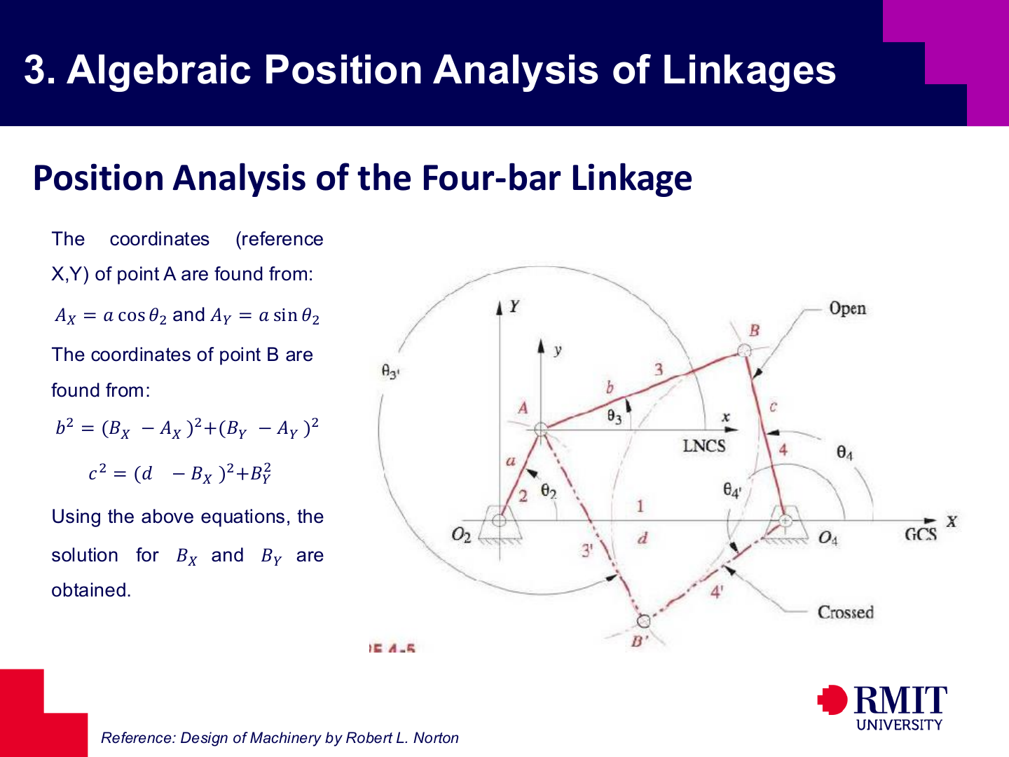
The algebraic method replaces the drawing process with coordinate equations.

Point $A$ is found from

\[\begin{aligned} A_X &= a \cos \theta_2, \\ A_Y &= a \sin \theta_2 \end{aligned}\]

Point $B$ is then constrained by the two link-length relations

\[\begin{aligned} b^2 &= (B_X - A_X)^2 + (B_Y - A_Y)^2, \\ c^2 &= (d - B_X)^2 + B_Y^2 \end{aligned}\]

These equations describe circles set by the coupler and rocker lengths. Solving them gives the unknown coordinates of $B$. The remaining link angles can then be found using trigonometry.

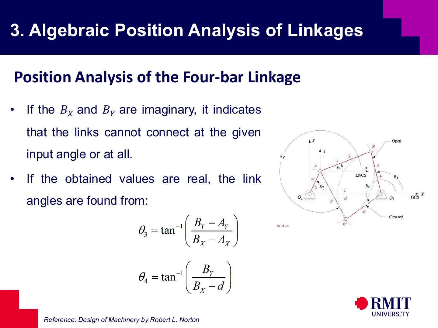
If the calculated values of $B_X$ and $B_Y$ are imaginary, the linkage cannot close at the chosen input angle. If the values are real, the remaining link angles can be found from the coordinates. More than one real solution may represent different assembly modes.

The two real solutions usually represent the open and crossed configurations. A possible configuration therefore depends on both the link lengths and whether the chosen input angle allows the linkage to close.

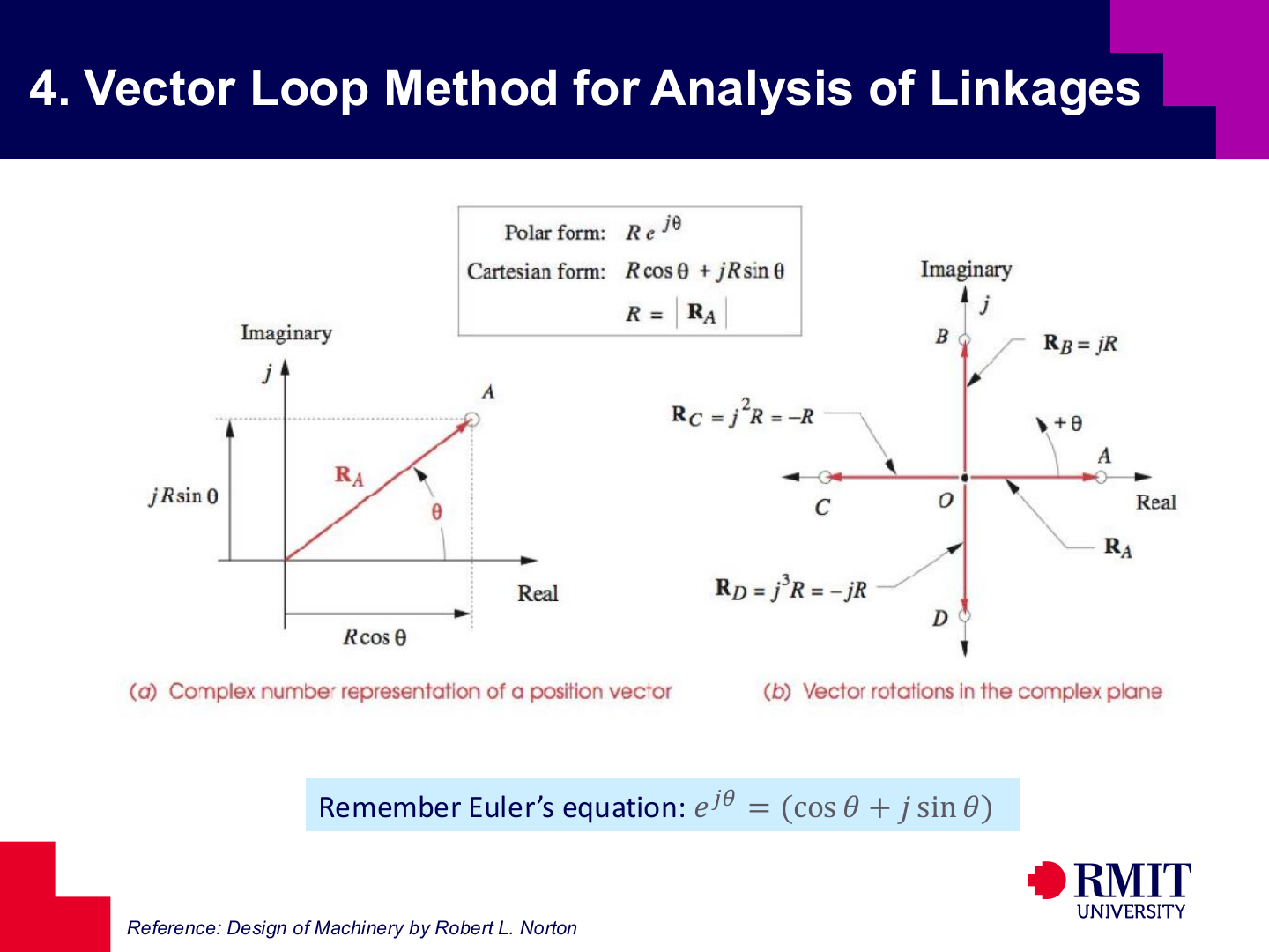
The vector-loop method represents each link as a vector. The vectors around a closed loop must add to zero. Writing them in complex form and using Euler’s relation $e^{j\theta} = \cos \theta + j \sin \theta$ changes the four-bar geometry into compact algebraic equations.

The same loop equation can later be differentiated to find velocity and acceleration without creating a new model of the mechanism.

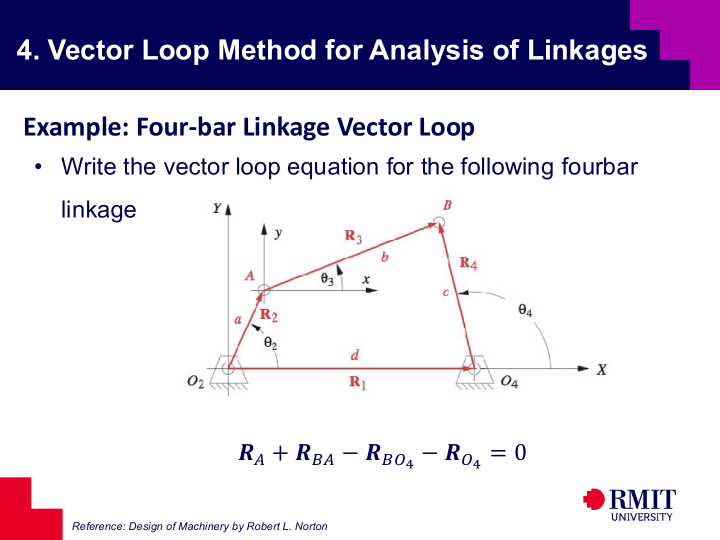
The main loop equation for the four-bar is $\mathbf{R}_{A} + \mathbf{R}_{BA} - \mathbf{R}_{BO_4} - \mathbf{R}_{O_4} = 0.$ Moving around the loop from the ground pivot and back to the starting point gives zero total displacement.

Every correct position must satisfy this equation. The vector form includes the geometry, closure and sign convention in one equation.

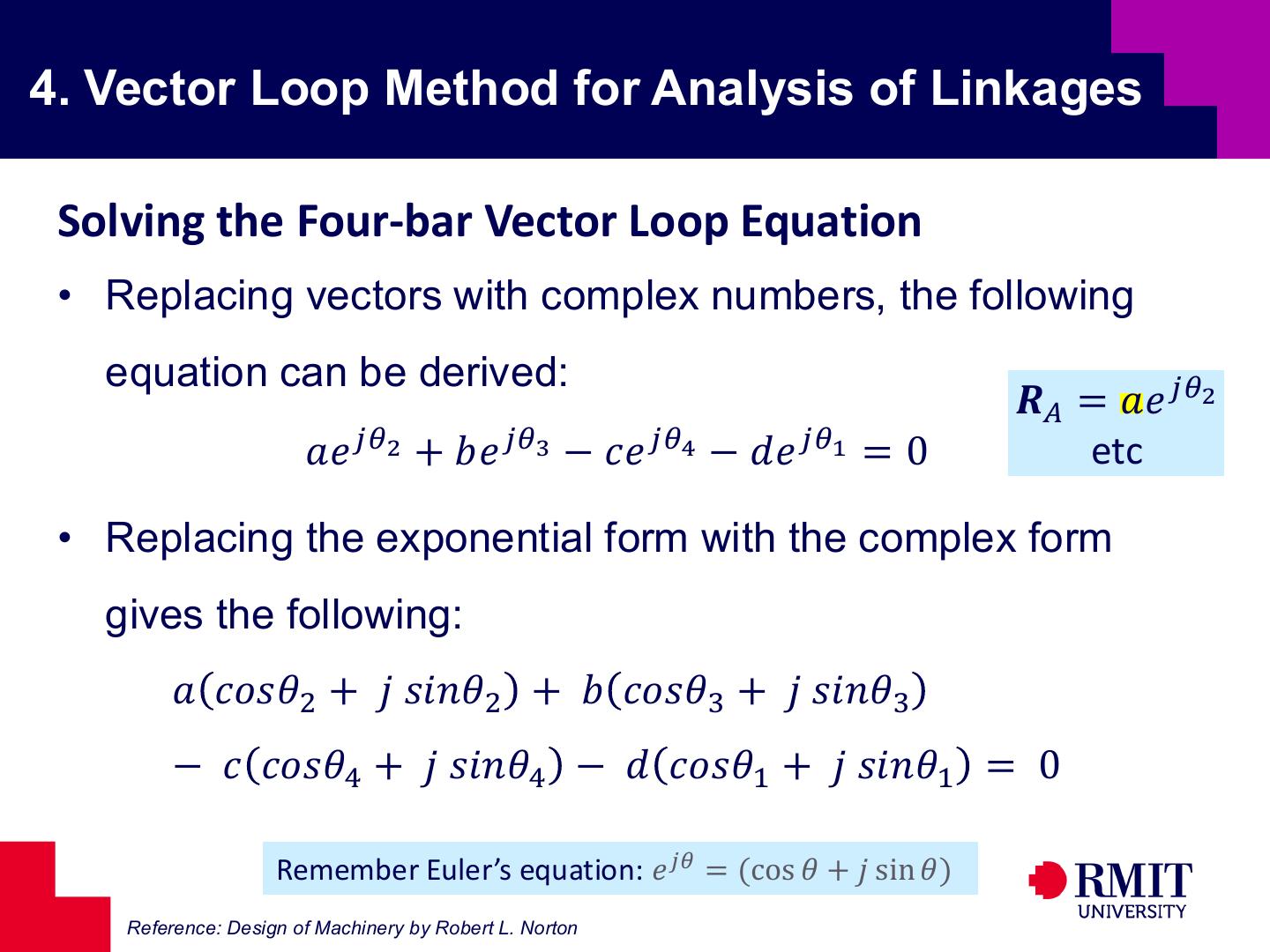
Replacing each vector with its complex polar form produces

\[a e^{j\theta_2} + b e^{j\theta_3} - c e^{j\theta_4} - d e^{j\theta_1} = 0.\]

Expanding the exponentials into sines and cosines converts the geometric closure problem into

\[a(\cos\theta_2 + j\sin\theta_2)+b(\cos\theta_3 + j\sin\theta_3)-c(\cos\theta_4 + j\sin\theta_4)-d(\cos\theta_1 + j\sin\theta_1)=0.\]

The vector equation can now be separated into scalar equations. The real part represents horizontal closure, and the imaginary part represents vertical closure.

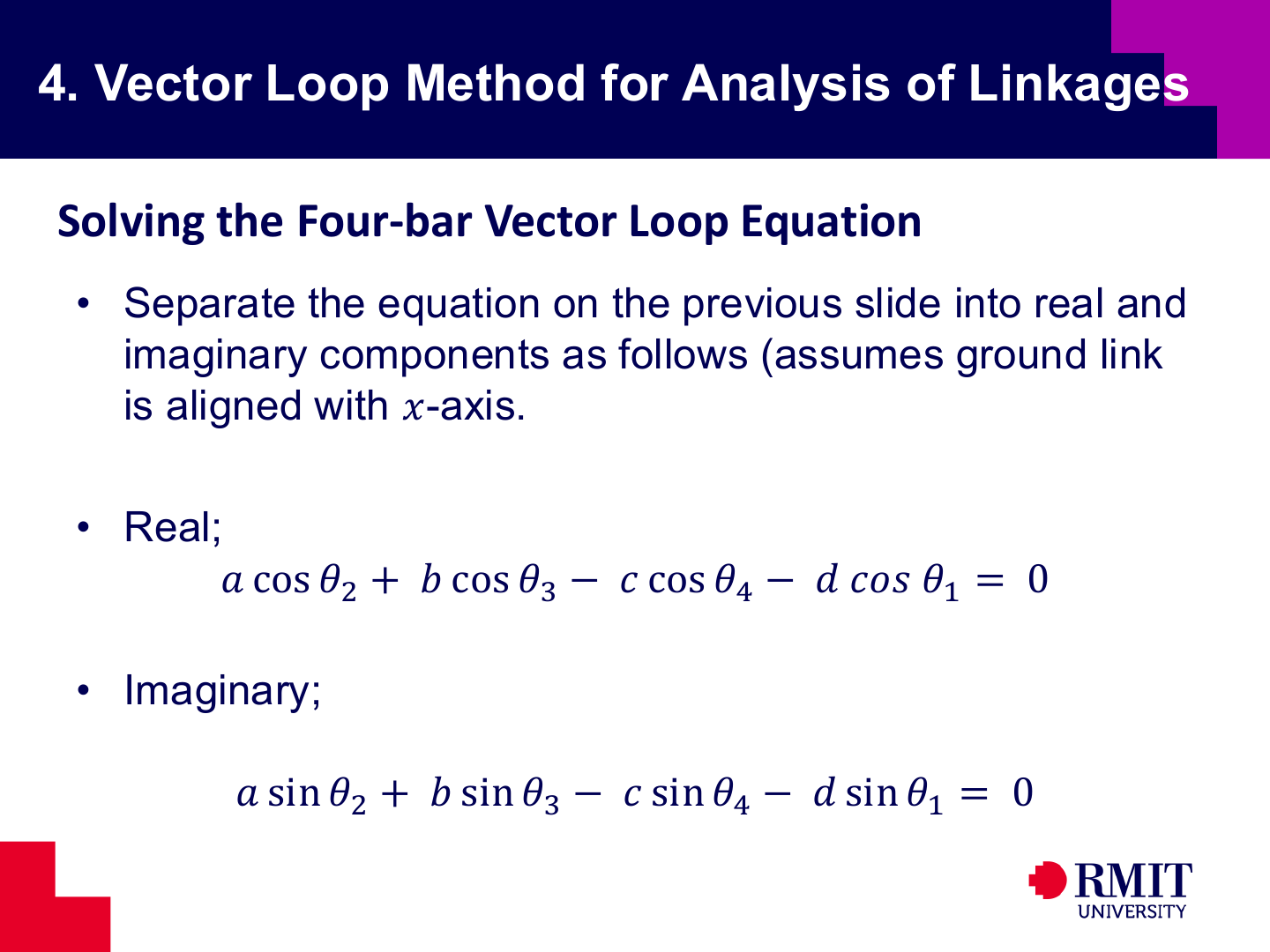
Separating the equation into real and imaginary parts gives the scalar closure relations

\[\begin{aligned} a\cos\theta_2 + b\cos\theta_3 - c\cos\theta_4 - d\cos\theta_1 &= 0, \\ a\sin\theta_2 + b\sin\theta_3 - c\sin\theta_4 - d\sin\theta_1 &= 0 \end{aligned}\]

If the ground link is aligned with the $x$-axis, then $\theta_1=0$, so the real equation contains $-d$ and the imaginary equation loses the ground-link term entirely.

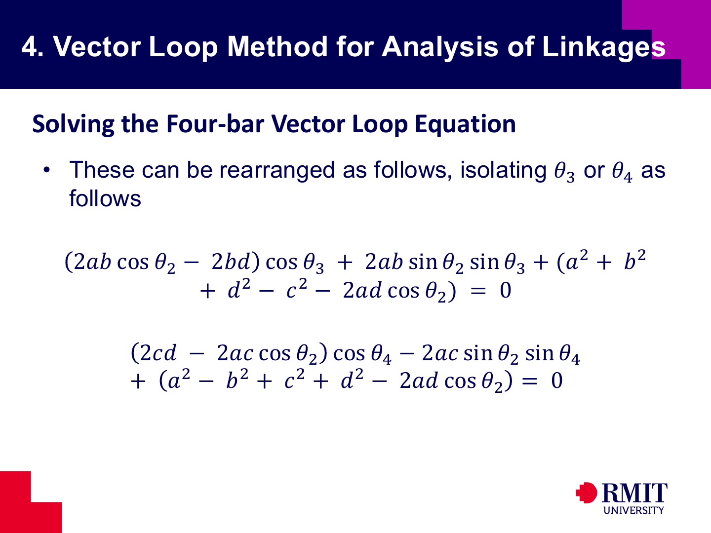
The next step is to rearrange the two scalar equations into a form involving only one unknown angle at a time:

\[\begin{aligned} (2ab\cos\theta_2 - 2bd)\cos\theta_3 + 2ab\sin\theta_2\sin\theta_3 + (a^2+b^2+d^2-c^2-2ad\cos\theta_2) &= 0, \\ (2cd-2ac\cos\theta_2)\cos\theta_4 - 2ac\sin\theta_2\sin\theta_4 + (a^2-b^2+c^2+d^2-2ad\cos\theta_2) &= 0 \end{aligned}\]

Each trigonometric equation now contains only one unknown angle.

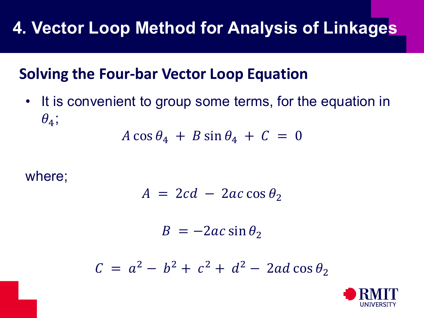
For the equation in $\theta_4$, it is convenient to define

\[\begin{aligned} A &= 2cd - 2ac\cos\theta_2, \\ B &= -2ac\sin\theta_2, \\ C &= a^2-b^2+c^2+d^2-2ad\cos\theta_2 \end{aligned}\]

so that the equation becomes $A\cos\theta_4 + B\sin\theta_4 + C = 0.$

This shorter form contains only $\theta_4$ and is ready for a standard trigonometric substitution.

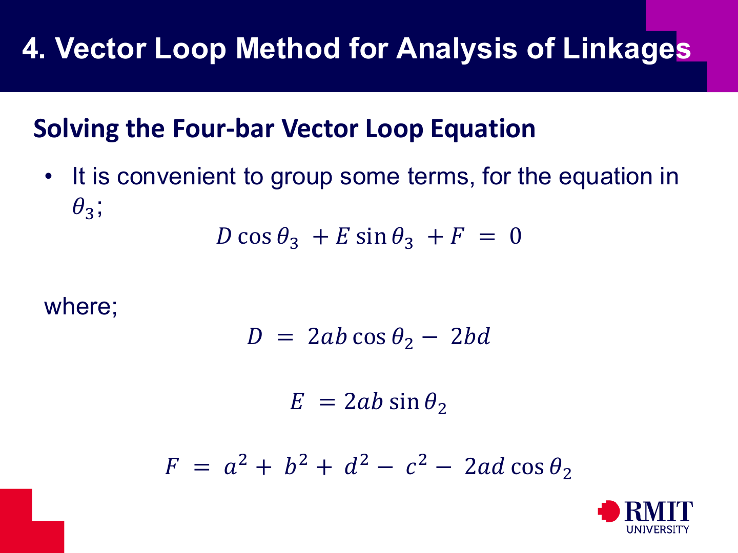
For the equation in $\theta_3$, define

\[\begin{aligned} D &= 2ab\cos\theta_2 - 2bd, \\ E &= 2ab\sin\theta_2, \\ F &= a^2+b^2+d^2-c^2-2ad\cos\theta_2 \end{aligned}\]

so that $D\cos\theta_3 + E\sin\theta_3 + F = 0.$

Like the previous equation, it has one cosine term, one sine term and one constant term.

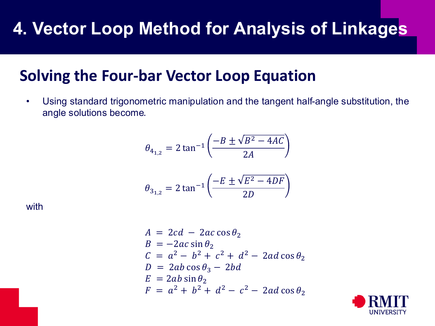
The final analytical step is to apply a tangent half-angle substitution, such as

\[\begin{aligned} t &= \tan\left(\frac{\theta}{2}\right), \\ \cos\theta &= \frac{1-t^2}{1+t^2}, \\ \sin\theta &= \frac{2t}{1+t^2} \end{aligned}\]

Substituting this into an equation of the form $A\cos\theta + B\sin\theta + C = 0$ produces a quadratic in $t$, $(C-A)t^2 + 2Bt + (A+C) = 0,$

First solve this equation for the possible values of $t$. Then convert each real root back to an angle using $\theta = 2\tan^{-1}(t)$.

Two real roots usually give two possible assembly configurations. Imaginary roots mean that the linkage cannot close.

The full derivation is worked through in the notes on Vector Loop Position Analysis.

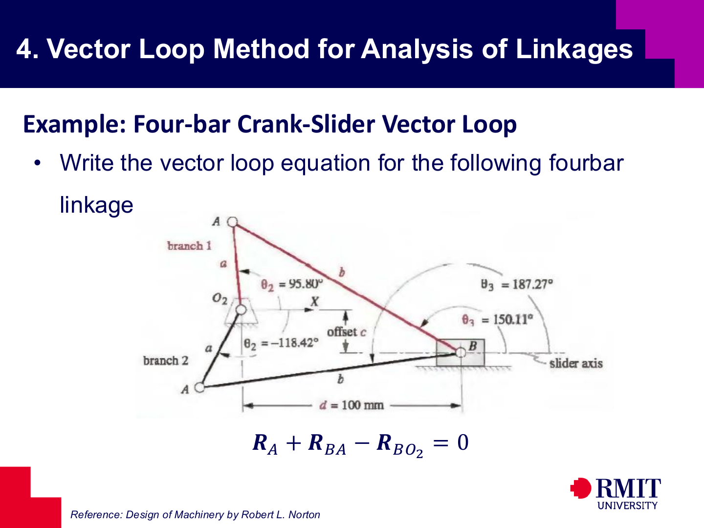
The same vector-loop method applies to the four-bar crank-slider when slider position is a linear unknown. With the sign convention used here, the closure equation is $\mathbf{R}_{A} + \mathbf{R}_{BA} - \mathbf{R}_{BO_2} = 0.$ It connects the crank, coupler and slider-position vectors.

Here, $c$ is the signed vertical offset of the slider axis relative to $O_2$: $c<0$ when the slider axis is below $O_2$, and $c>0$ when it is above $O_2$. Therefore, $\mathbf{R}_{BO_2}=d+jc$.

In complex form, with the same convention for $\theta_3$, this becomes $a e^{j\theta_2} - b e^{j\theta_3} - (d + jc) = 0,$ so the real and imaginary parts give

\[\begin{aligned} a\cos\theta_2 - b\cos\theta_3 - d &= 0, \\ a\sin\theta_2 - b\sin\theta_3 - c &= 0 \end{aligned}\]

The method is therefore unchanged in structure: write the loop equation, expand it, separate components, and solve for the unknown position variables.

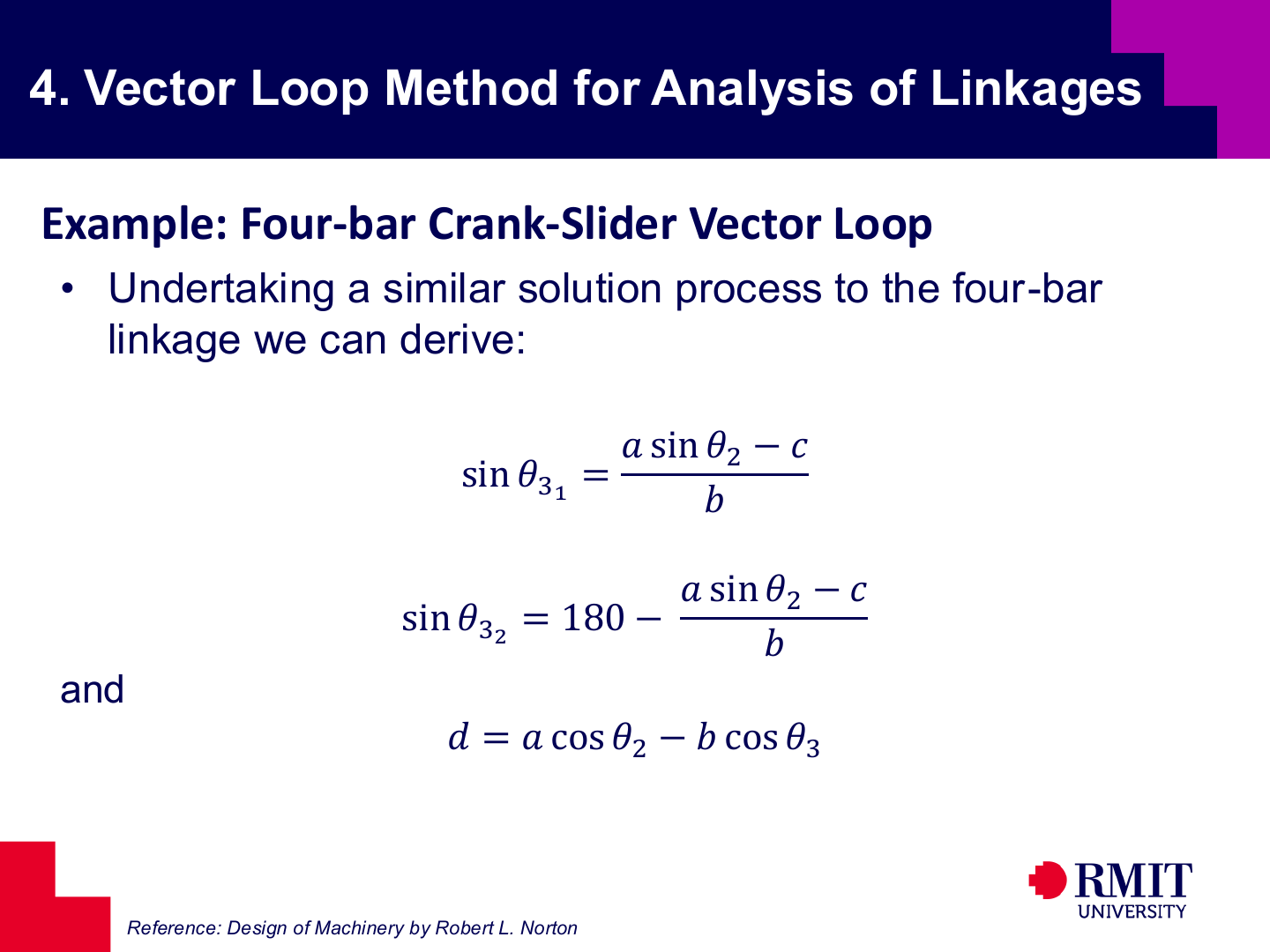
For the crank-slider, the imaginary equation can be solved first to obtain the coupler-angle branches: $\sin\theta_3=\frac{a\sin\theta_2-c}{b}.$

This gives two assembly modes. The main inverse-sine value gives one mode, and the supplementary angle gives the other. They represent the open and crossed configurations.

After finding both values of $\theta_3$, calculate the slider position for each one using the real equation. Select the value of $d$ that matches the sign convention and chosen assembly mode.

Once the appropriate value of $\theta_3$ has been chosen, the slider position follows from the real equation: $d = a\cos\theta_2 - b\cos\theta_3.$

The four-bar and crank-slider therefore use the same vector-loop process. The crank-slider has one unknown angle and one unknown linear position.

[For Illustration Only]

[For Illustration Only]

[For Illustration Only]

[For Illustration Only]

[For Illustration Only]

[For Illustration Only]

[For Illustration Only]

[For Illustration Only]

Velocity can be analysed using graphical, algebraic, complex-number, vector-loop or numerical methods. Each method represents the same kinematic constraints in a different way.

The vector-loop method gives a direct path from known positions to velocities. The same method can then be extended to acceleration analysis.

Velocity analysis starts after the mechanism position is known. It finds the angular velocities of the links and the linear velocities of selected points.

Acceleration analysis needs these velocities, and dynamic force calculations need acceleration. Velocity analysis therefore connects position analysis to later force and stress calculations.

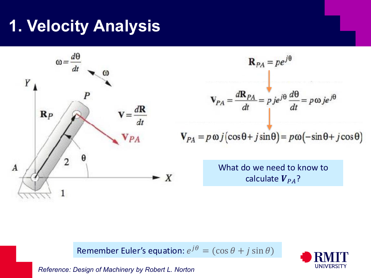
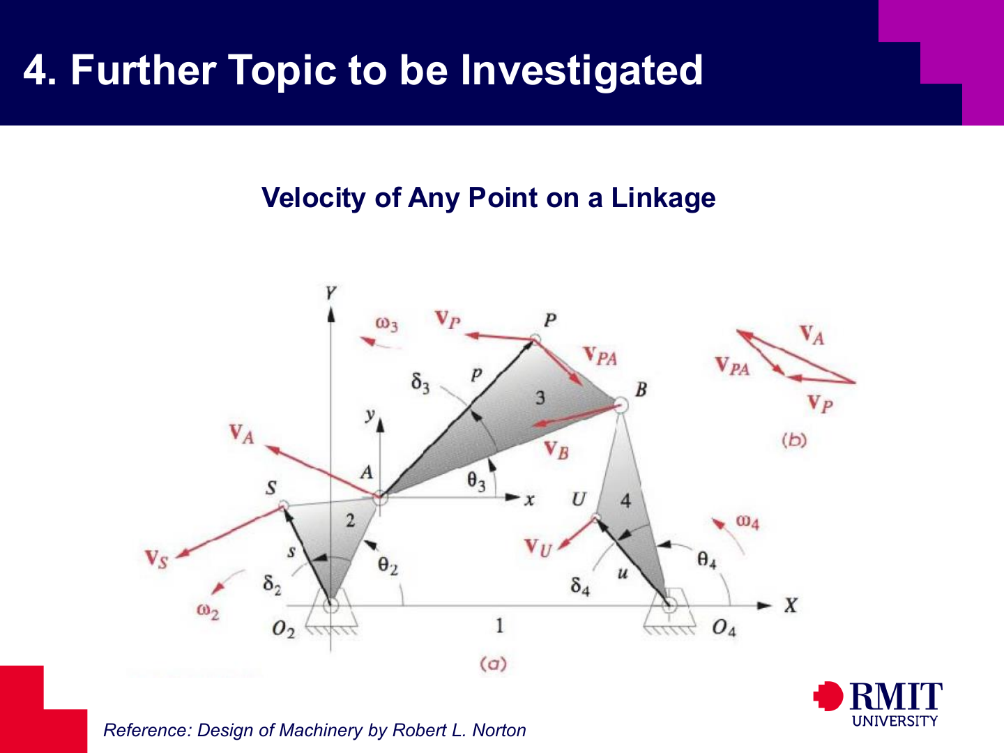
For a point $P$ on a rotating link relative to point $A$, the position vector is written as $\mathbf{R}_{PA}=p e^{j\theta}.$

Differentiating with respect to time gives

\[\mathbf{V}_{PA}=\frac{d\mathbf{R}_{PA}}{dt}=j p \omega e^{j\theta}=p\omega(-\sin\theta+j\cos\theta)\]

The magnitude is therefore $p\omega$, and the direction is perpendicular to the radius vector. The required inputs are the distance $p$, the angular position $\theta$, and the angular velocity $\omega$.

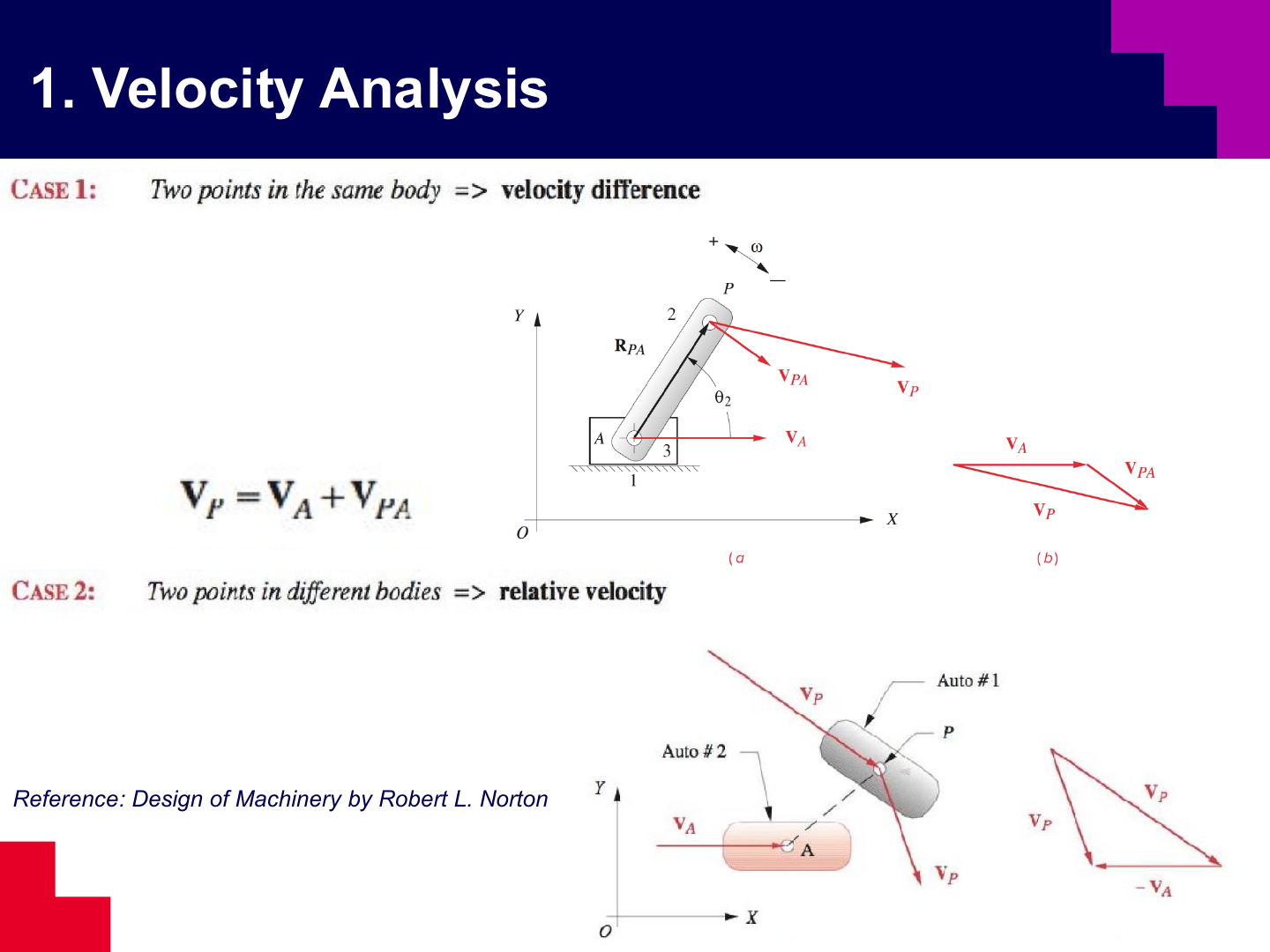
When two points lie on the same rigid body, the appropriate relation is the velocity-difference equation $\mathbf{V}_{P}=\mathbf{V}_{A}+\mathbf{V}_{PA}.$

In this equation, $\mathbf{V}_{PA}$ is the velocity caused by rotation between the two points.

When two points are on different bodies, one rigid-body velocity equation cannot connect them. Their velocities must satisfy the joint or contact constraint. For example, a shared pin has the same velocity when calculated from either link.

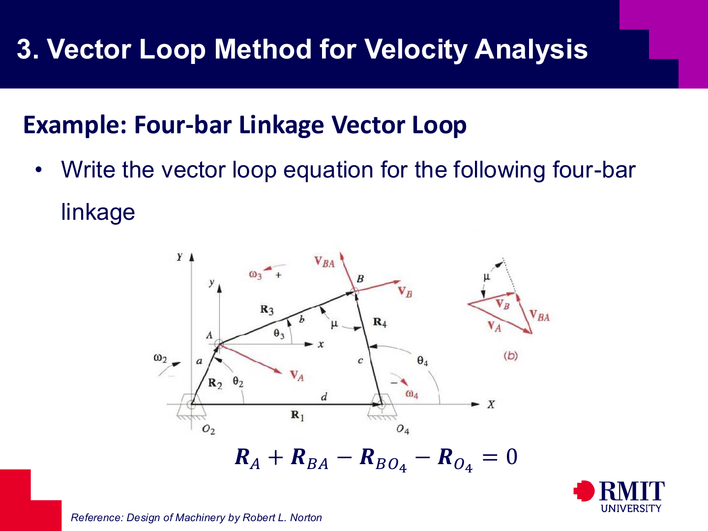
Velocity analysis for the four-bar begins from the same loop equation used in the position analysis, $\mathbf{R}_{A}+\mathbf{R}_{BA}-\mathbf{R}_{BO_4}-\mathbf{R}_{O_4}=0.$

Once the position equation is known, differentiating it gives the velocity equation directly.

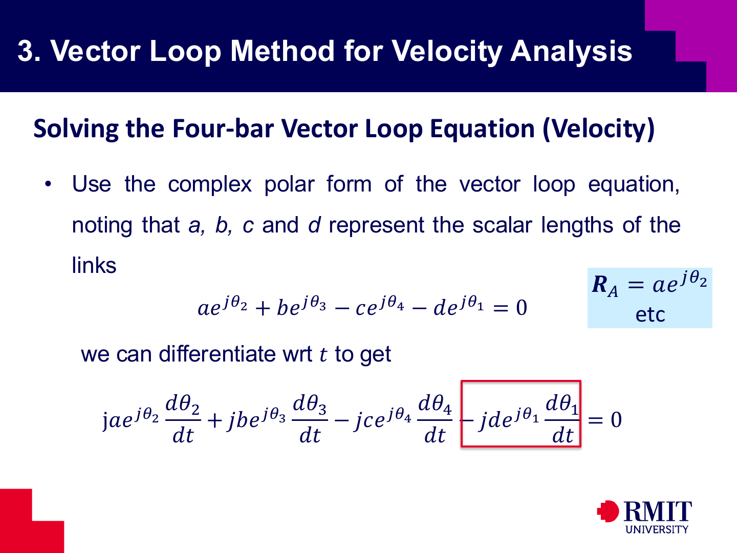
Replacing the vectors with their complex polar forms gives $a e^{j\theta_2}+b e^{j\theta_3}-c e^{j\theta_4}-d e^{j\theta_1}=0.$

Differentiating with respect to time produces a velocity loop involving the angular rates of the moving links:

\[\begin{aligned} j a e^{j\theta_2}\frac{d\theta_2}{dt} &+j b e^{j\theta_3}\frac{d\theta_3}{dt} \\ &-j c e^{j\theta_4}\frac{d\theta_4}{dt} \\ &-j d e^{j\theta_1}\frac{d\theta_1}{dt}=0 \end{aligned}\]

The term containing $\theta_1$ comes from differentiating the ground-link vector. In the general form it is kept so that the differentiation is shown consistently for all four links.

For the usual four-bar reference frame, however, the ground link is fixed and aligned with the $x$-axis, so $\theta_1$ is constant and therefore $\frac{d\theta_1}{dt}=0.$

That makes the ground-link term vanish, leaving only the moving-link terms in the velocity equation.

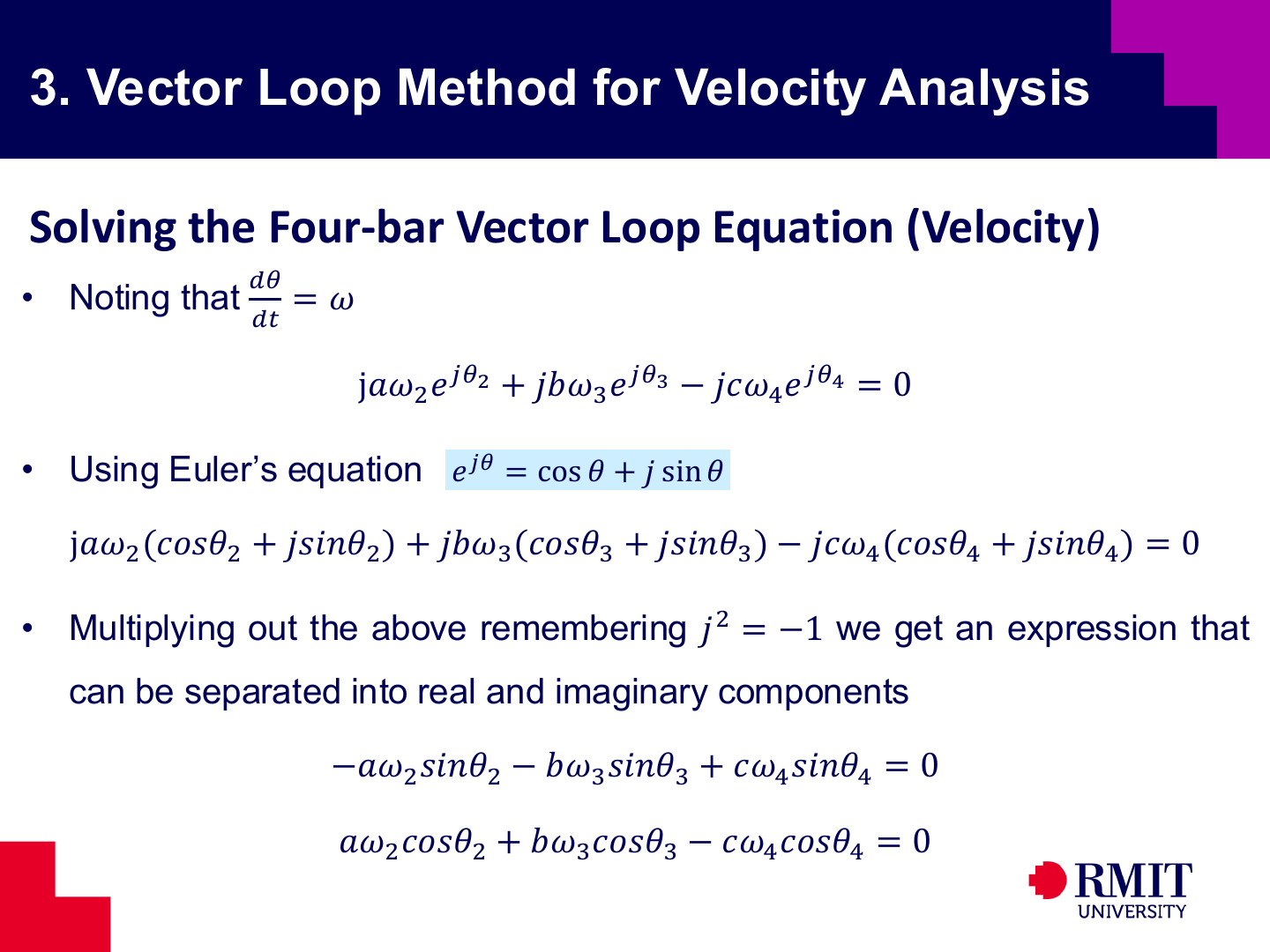
With $\omega=d\theta/dt$ and Euler’s relation $e^{j\theta}=\cos\theta+j\sin\theta$, the differentiated loop becomes $j a \omega_2 e^{j\theta_2}+j b \omega_3 e^{j\theta_3}-j c \omega_4 e^{j\theta_4}=0.$

Expanding and separating into components gives the scalar equations

\[\begin{aligned} -a\omega_2\sin\theta_2-b\omega_3\sin\theta_3+c\omega_4\sin\theta_4 &= 0, \\ a\omega_2\cos\theta_2+b\omega_3\cos\theta_3-c\omega_4\cos\theta_4 &= 0 \end{aligned}\]

These two equations are then solved for the unknown angular velocities $\omega_3$ and $\omega_4$.

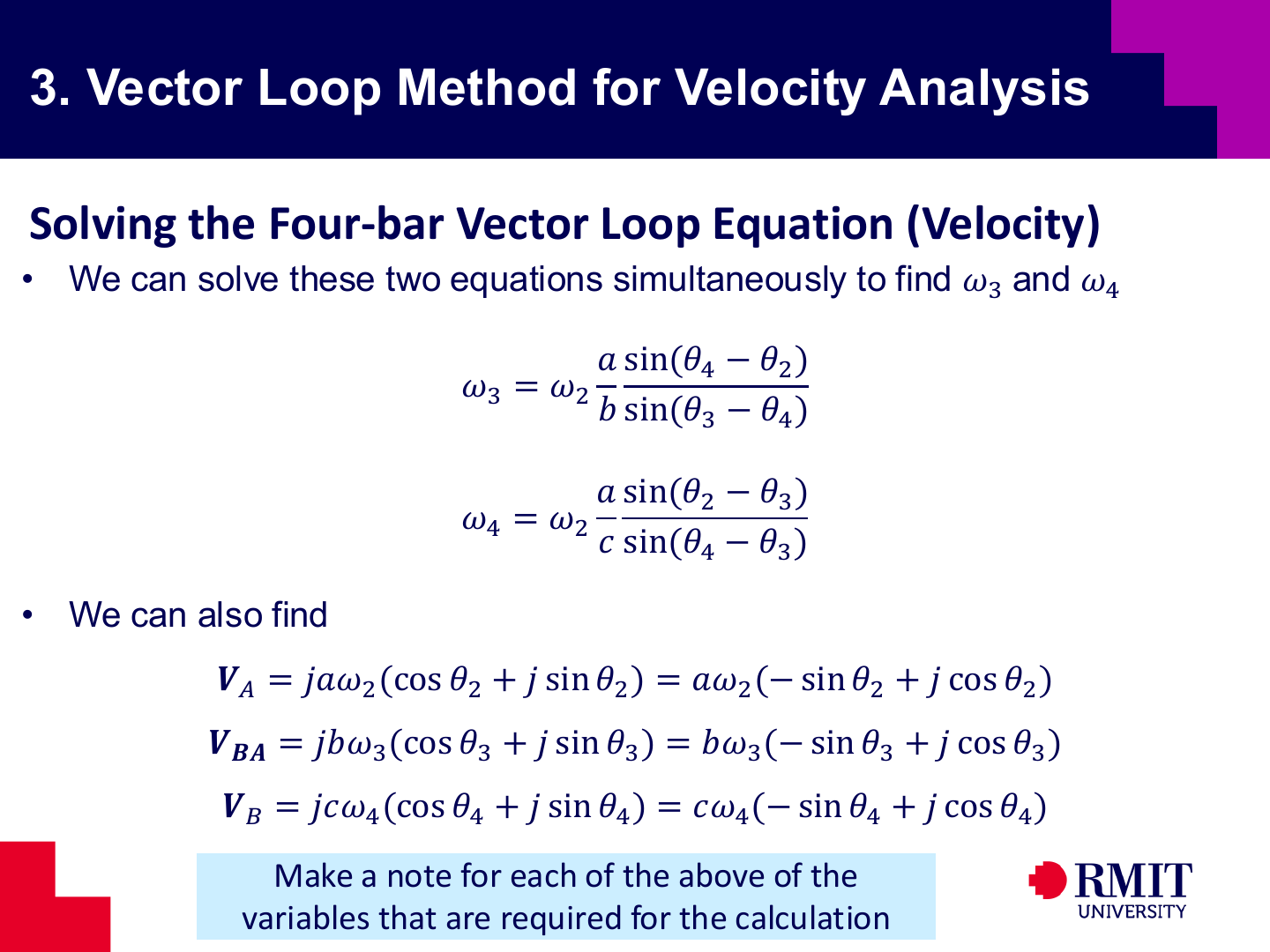
Solving the two scalar equations simultaneously gives

\[\begin{aligned} \omega_3 &= \omega_2\frac{a\sin(\theta_4-\theta_2)}{b\sin(\theta_3-\theta_4)}, \\ \omega_4 &= \omega_2\frac{a\sin(\theta_2-\theta_3)}{c\sin(\theta_4-\theta_3)} \end{aligned}\]

These expressions are valid only after the position analysis has supplied the current values of $\theta_3$ and $\theta_4$.

Once the angular velocities are known, point velocities follow directly from

\[\begin{aligned} \mathbf{V}_A &= a\omega_2(-\sin\theta_2+j\cos\theta_2), \\ \mathbf{V}_{BA} &= b\omega_3(-\sin\theta_3+j\cos\theta_3), \\ \mathbf{V}_B &= c\omega_4(-\sin\theta_4+j\cos\theta_4) \end{aligned}\]

These results are velocity vectors. If only speed is required, use the magnitude of the vector. A negative angular velocity shows the direction of rotation, not a negative speed.

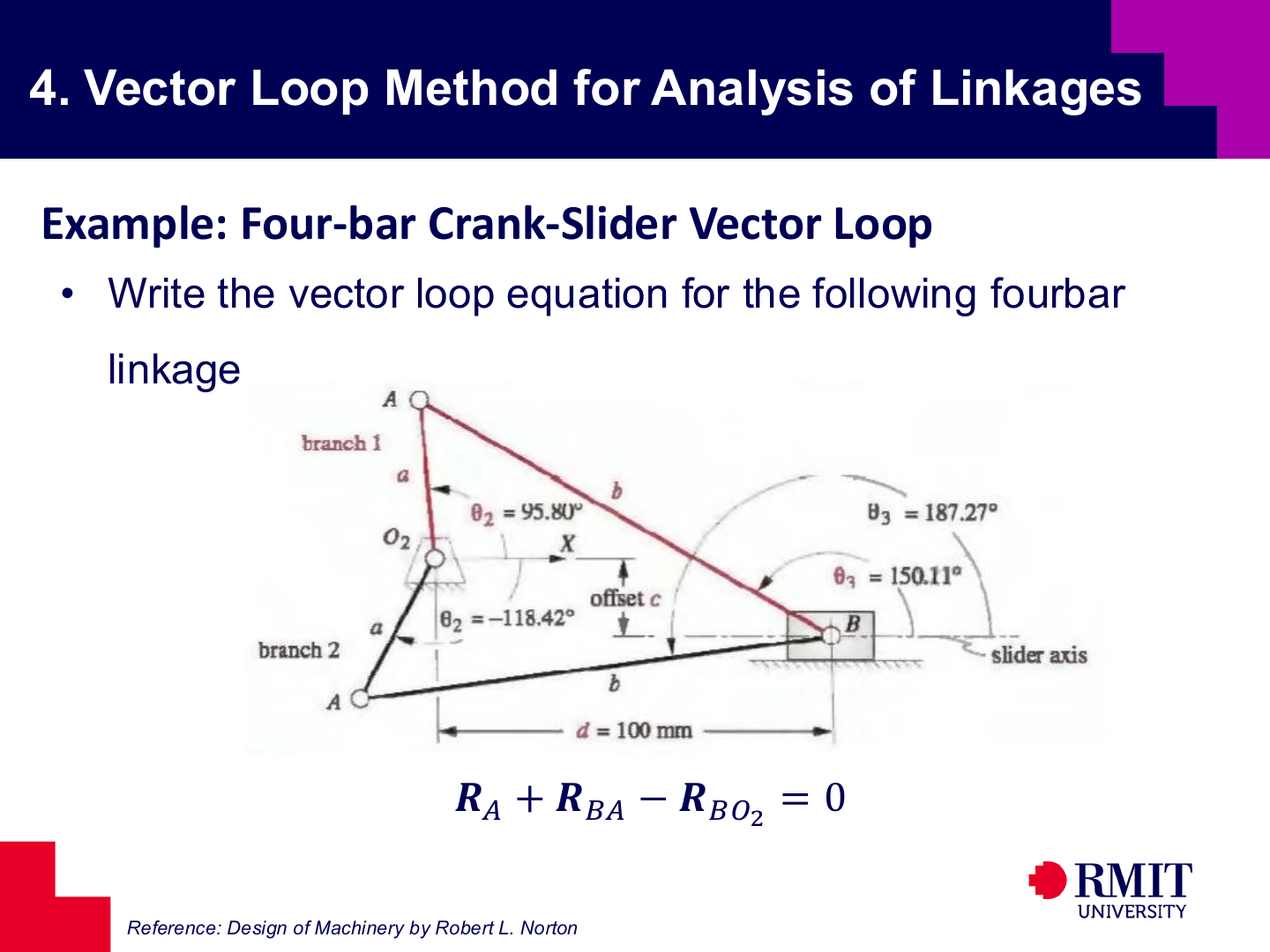
Crank-slider velocity analysis begins with the loop equation $\mathbf{R}_{A}+\mathbf{R}_{BA}-\mathbf{R}_{BO_2}=0.$ Start with the known position, differentiate with respect to time, and separate the result into scalar equations for the unknown velocities at that position.

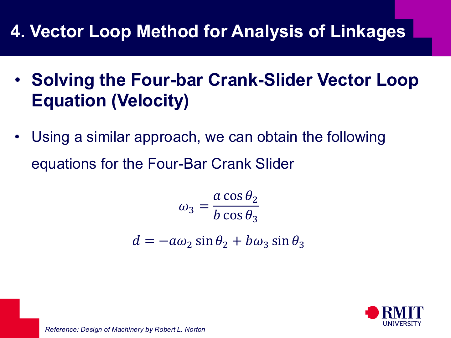
For the four-bar crank-slider, the velocity relations are

\[\begin{aligned} \omega_3 &= \frac{a\cos\theta_2}{b\cos\theta_3}\omega_2, \\ \dot d &= -a\omega_2\sin\theta_2+b\omega_3\sin\theta_3 \end{aligned}\]

The first equation gives the coupler angular velocity, while the second gives the slider speed. The transfer from the four-bar is therefore direct: the same differentiated loop-closure logic is used, but one unknown is now linear rather than angular.

[For Illustration Only]

[For Illustration Only]

[For Illustration Only]

[For Illustration Only]

[For Illustration Only]

[For Illustration Only]

Acceleration analysis follows velocity analysis. Differentiating the velocity equations gives the linear and angular accelerations needed for dynamic force and stress calculations.

The same vector loop is used. The acceleration equations contain tangential terms related to angular acceleration and normal terms related to angular velocity squared.

Dynamic force depends directly on acceleration. Knowing the acceleration of each link and point allows the inertia forces and resulting component stresses to be calculated.

Rigid-body acceleration has two useful components. One shows how quickly a point speeds up along its path. The other points towards the centre of the curved path.

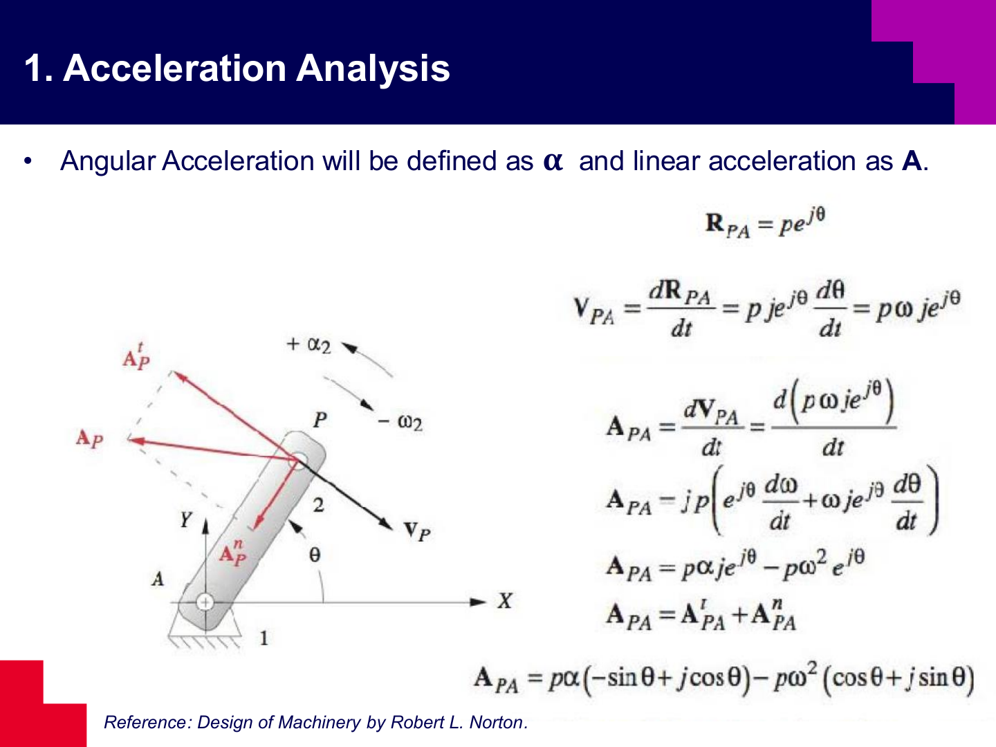
Angular acceleration is denoted by $\alpha$, while linear acceleration is denoted by $\mathbf{A}$.

The equations contain rotational and translational effects together. Clear notation helps distinguish tangential terms from normal terms.

For a point at radius $r$ on a rotating link, tangential acceleration has magnitude $r\alpha$. Normal, or centripetal, acceleration has magnitude $r\omega^2$ and points towards the centre of rotation.

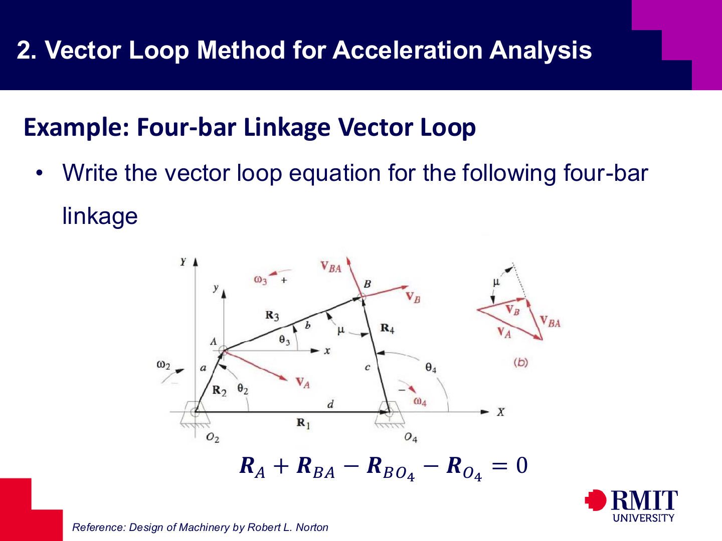
The acceleration calculation uses the same four-bar geometry and vector loop as the position and velocity calculations. The unknown values are now angular accelerations and point accelerations.

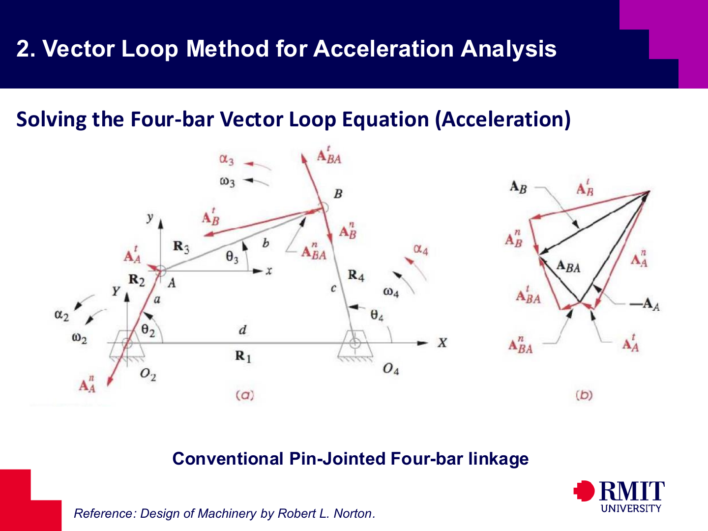
Each point acceleration is separated into a tangential component related to angular acceleration and a normal component related to angular velocity squared. The vector diagram shows how these components combine to close the acceleration loop.

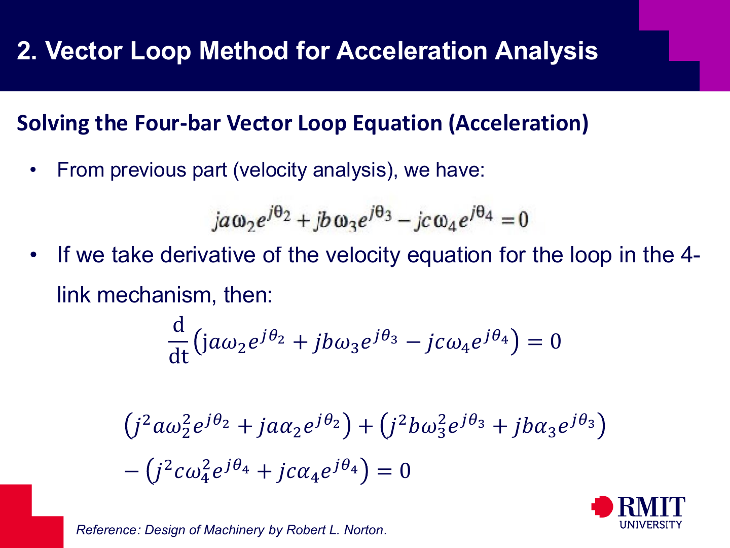
Start with the velocity loop $j a \omega_2 e^{j\theta_2} + j b \omega_3 e^{j\theta_3} - j c \omega_4 e^{j\theta_4} = 0.$ Differentiating it with respect to time produces angular-acceleration terms and centripetal terms containing $\omega^2$. In complex form, differentiating $j\omega e^{j\theta}$ gives a $j\alpha e^{j\theta}$ term and a $-\omega^2 e^{j\theta}$ term.

That is why acceleration analysis contains both tangential and normal components.

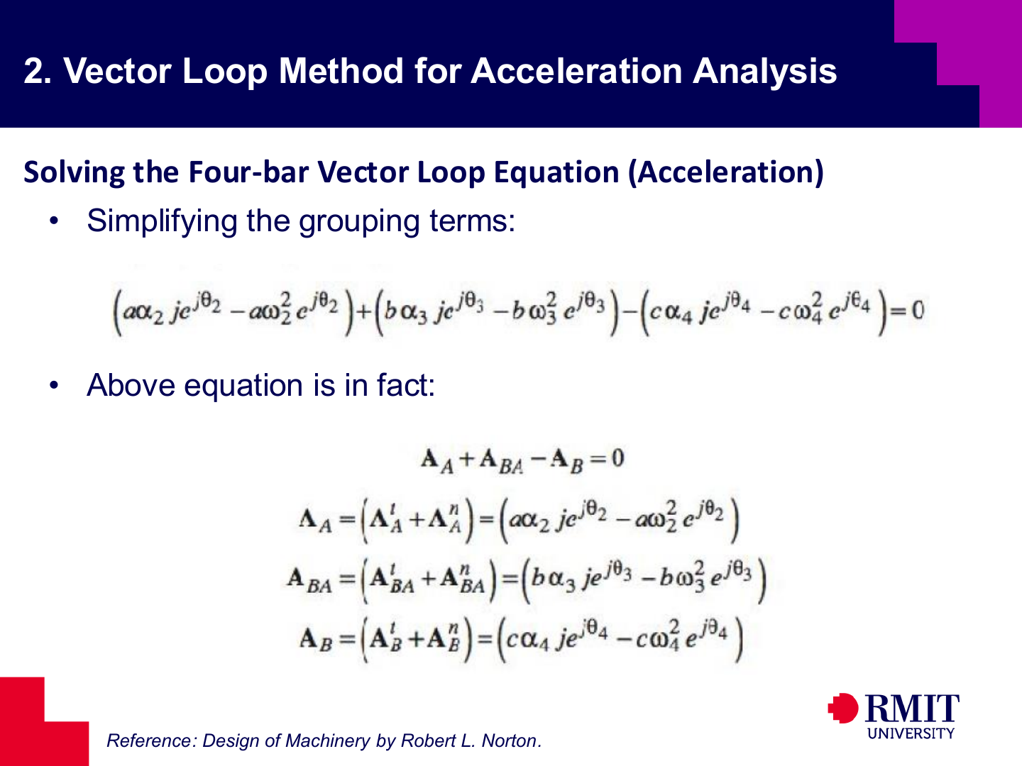
After grouping the terms, each link has a tangential part containing $\alpha$ and a normal part containing $\omega^2$. The acceleration loop is $\mathbf{A}_{A} + \mathbf{A}_{BA} - \mathbf{A}_{B} = 0.$

This is the acceleration version of loop closure for the four-bar.

Each vector combines a tangential component and a normal component pointing towards the centre of the curved path.

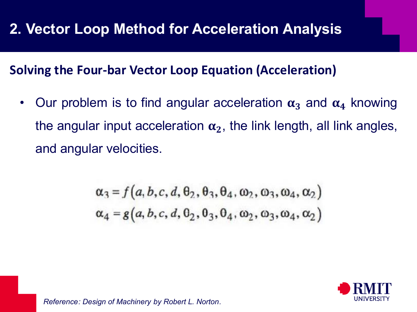
The aim is to find the unknown angular accelerations $\alpha_3$ and $\alpha_4$. The known values are the input angular acceleration $\alpha_2$, link lengths, current link angles and angular velocities found during velocity analysis.

Acceleration analysis therefore needs the results of both position and velocity analysis.

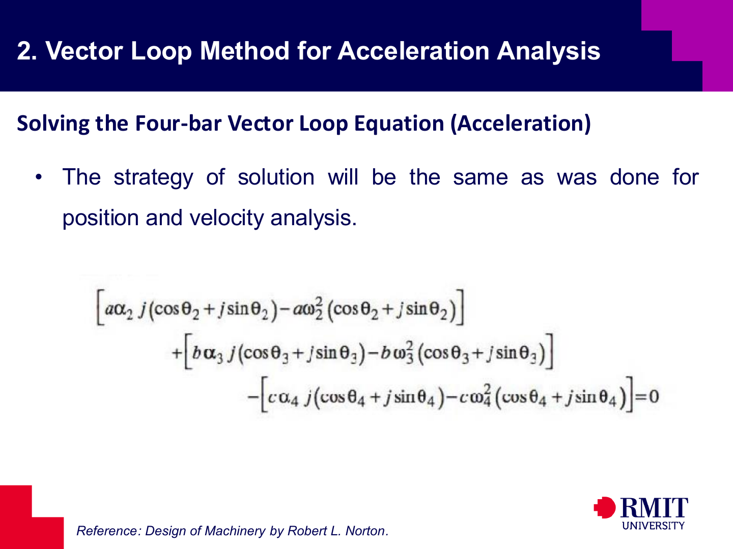
Use the same process as before. Expand the complex equation, separate the real and imaginary parts, and solve the two scalar equations together. The same vector-loop structure works for position, velocity and acceleration.

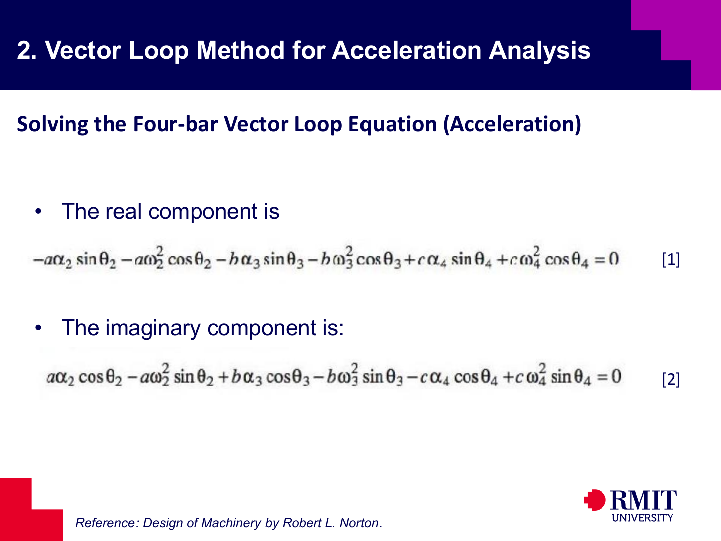
Separate the acceleration loop into real and imaginary equations. These equations contain tangential terms in $\alpha_2$, $\alpha_3$ and $\alpha_4$, and normal terms in $\omega_2^2$, $\omega_3^2$ and $\omega_4^2$. Together, they can be solved for the unknown angular accelerations.

When the geometry and angular velocities are known, the equations are linear in $\alpha_3$ and $\alpha_4$. Substituting the known values gives two simultaneous linear equations for these two unknowns.

Written explicitly, the two scalar acceleration equations are

\[\begin{aligned} -a\alpha_2\sin\theta_2-a\omega_2^2\cos\theta_2-b\alpha_3\sin\theta_3-b\omega_3^2\cos\theta_3+c\alpha_4\sin\theta_4+c\omega_4^2\cos\theta_4 &= 0, \\ a\alpha_2\cos\theta_2-a\omega_2^2\sin\theta_2+b\alpha_3\cos\theta_3-b\omega_3^2\sin\theta_3-c\alpha_4\cos\theta_4+c\omega_4^2\sin\theta_4 &= 0 \end{aligned}\]

These are solved simultaneously for $\alpha_3$ and $\alpha_4$.

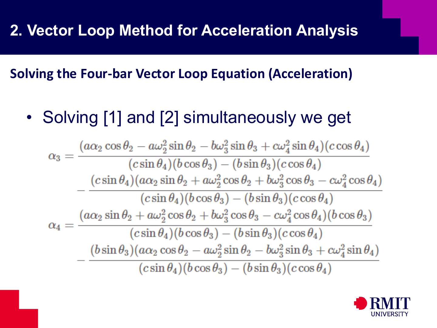
Solving the two component equations together gives $\alpha_3$ and $\alpha_4$. The formulas are longer than the velocity formulas, but the same principle applies. The known geometry and input motion determine the motion of the other links.

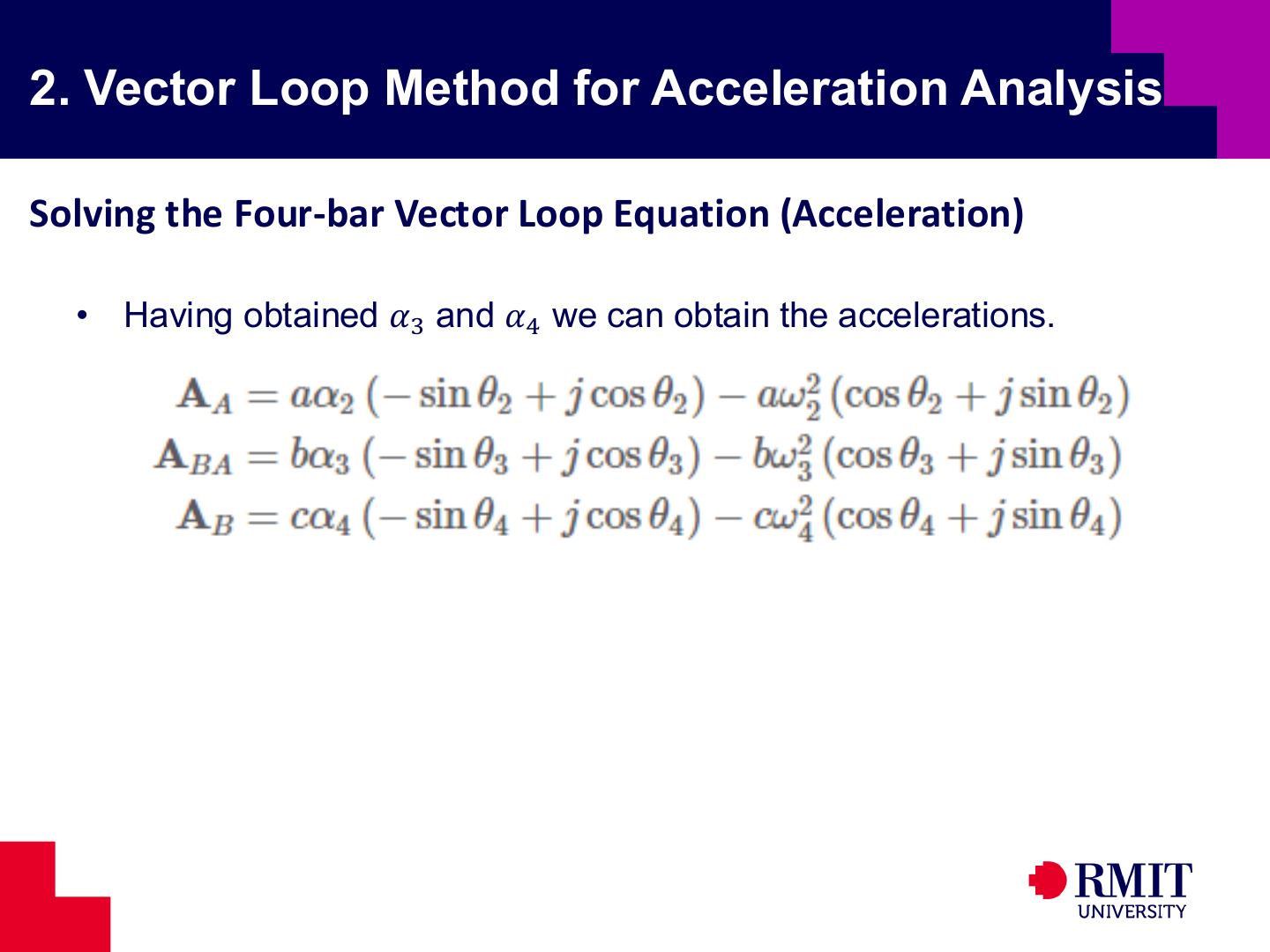
After finding $\alpha_3$ and $\alpha_4$, use the complex rigid-body equations to find point accelerations. Each equation combines a tangential term containing $\alpha$ and a normal term containing $\omega^2$.

For the four-bar linkage, the principal point accelerations may be written as

\[\begin{aligned} \mathbf{A}_A &= a\alpha_2(-\sin\theta_2+j\cos\theta_2)-a\omega_2^2(\cos\theta_2+j\sin\theta_2), \\ \mathbf{A}_{BA} &= b\alpha_3(-\sin\theta_3+j\cos\theta_3)-b\omega_3^2(\cos\theta_3+j\sin\theta_3), \\ \mathbf{A}_B &= c\alpha_4(-\sin\theta_4+j\cos\theta_4)-c\omega_4^2(\cos\theta_4+j\sin\theta_4) \end{aligned}\]

The real parts give the $x$-components and the imaginary parts give the $y$-components of the corresponding acceleration vectors. For example, if

\[\mathbf{A}_A = A_{Ax} + jA_{Ay},\]

then $A_{Ax}$ is the real part of $\mathbf{A}_A$ and $A_{Ay}$ is the imaginary part.

These point accelerations are used to calculate dynamic loads on pins, links, joints and connected components.

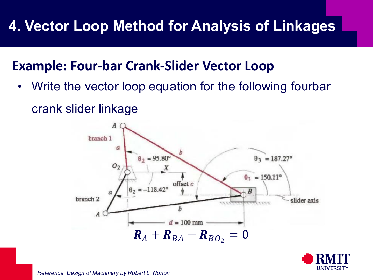
The crank-slider uses the same loop-closure rule as the four-bar, but one end point must remain on the slider axis. The loop $\mathbf{R}_{A}+\mathbf{R}_{BA}-\mathbf{R}_{BO_2}=0$ connects the crank, coupler and slider-position vectors.

Because point $B$ must follow the guide, its position is a linear distance along the slider axis instead of a second link angle. This is the main geometric difference from the four-bar.

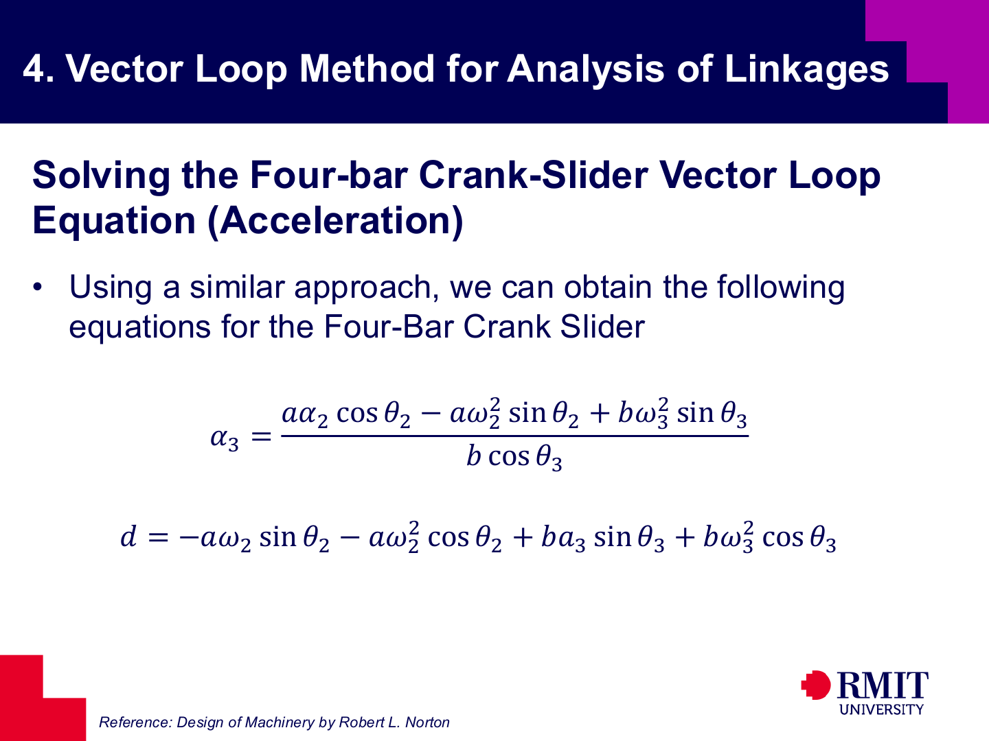
Crank-slider acceleration analysis follows the same sequence as four-bar analysis. Position analysis gives the current geometry. Velocity analysis gives $\omega_3$ and slider speed. Differentiating again gives coupler angular acceleration and slider acceleration.

The resulting acceleration relations are

\[\begin{aligned} \alpha_3 &= \frac{a\alpha_2\cos\theta_2-a\omega_2^2\sin\theta_2+b\omega_3^2\sin\theta_3}{b\cos\theta_3}, \\ \ddot d &= -a\alpha_2\sin\theta_2-a\omega_2^2\cos\theta_2+b\alpha_3\sin\theta_3+b\omega_3^2\cos\theta_3 \end{aligned}\]

The first equation gives the angular acceleration of the coupler, and the second gives the linear acceleration of the slider along its guide.

[For Illustration Only]

[For Illustration Only]

[For Illustration Only]

[For Illustration Only]

Knowledge Check